
![]()
Multidimensional Statistical Patterns Observed on Water Drops Corona Discharge Pictures
Raveloson, Faniry1; Roussel, Jérémie1; Vandanjon, Laurent2*; de la Bardonnie,Hugues1
1 Laboratory LIMEC, 24 rue du Général Ferrié, 31500 Toulouse, France
2 Laboratory of Marine Biotechnology and Chemistry (LBCM), University Bretagne Sud (UBS), EMR CNRS 6076, IUEM, Campus Tohannic, 56000 Vannes, France
*Corresponding author: laurent.vandanjon@univ-ubs.fr
Keywords: Corona effect, machine learning algorithms, random forest, K-Nearest Neighbors (KNN), gradient Boost, decision tree, naive Bayes
Submitted: June 26, 2023
Reviewed: September 28, 2023
Accepted: October 10, 2023
Published: March 5, 2024
Abstract
Macroscopic corona images of droplets of different kinds of water were examined by collecting dozens of image parameters. A statistical comparison of these parameters using Data Science (machine learning) algorithms allowed us to differentiate water types with significant accuracy. The ability to differentiate water types using macroscopic corona imaging combined with machine learning algorithms presents topics for further studies.
Introduction
The Corona effect, the electrical discharge caused by the ionization of the air surrounding a conductor carrying a high voltage, began to be studied at the beginning of the 20th century with the empiric work of F.W. Peek in 1929 (Hartmann, 1984), who characterized the threshold field to create the effect. It was then studied in the high-voltage industrial electrical network to understand the vibrations it induces in the cables (Farzaneh, 1986; Maaroufi, 1989) and then to monitor the resulting energy loss. In addition to the work aiming at reducing the corona effect in high-voltage transmission, research on this topic has led to commercial and industrial uses, such as the production of ozone (Chen and Davidson, 2002; Noll, 2002), the generation of charged surfaces (McGraw-Hill, 2007), and the treatment of certain polymer surfaces (Carley and Kitze, 1980; Tazuke et al, 1980), to name a few.
The use of the corona effect in imagery dates back to 1939, when Semyon Kirlian started to photograph the corona effect. It was then used by different people for scientific and non-scientific works. In the context of major breakthroughs in artificial intelligence in the last decades, it has been used in image analysis of large amounts of data to explore or revisit new fields of studies.
The goal of this study is to demonstrate that a Corona Effect Macroscopic Imaging (CEMI) technology, based on the well-known physical phenomena of corona discharge (Loeb, 1965), also called Electrophotonics, can be used to obtain a new type of information about the objects under study. The Electrophotonic DataPhoton System (EDS©) is the prototype device (Vieilledent et al, 2016) that we used in combination with machine learning algorithms to classify and differentiate between waters according to their properties. This study focuses on how to use macroscopic corona imaging on different types of water drops to extract corona parameters and so be able to identify and classify the drops according to a coherent multidimensional statistical approach using machine learning algorithms.
The Basis of Electrophotonics: Understanding Light and Water
Light
The hypothesis that light is composed of particles and therefore that it is corpuscular in nature was put forward by Sir Isaac Newton (Newton, 1952) in 1704 who, with his numerous experimental studies describing many physical phenomena, was able at the time to reject the wave theories of light of R. Hooke, C. Huygens, or L. Euler. In the 19th century, however, experimental observations such as the experiments on interference by T. Young (Young, 1802) or the discovery of polarization by E-L. Malus (Malus, 1811) suggested a wave nature to light. It is through the wave theory of A. Fresnel (Fresnel, 1826) and then finally the unification of electricity and magnetism by J.C. Maxwell (Maxwell, 1873) that light became then considered as a wave, more exactly an electromagnetic wave.
At the end of the 19th century, with the work of Max Planck and his hypothesis on the energy quantum (Planck, 1900), the classical vision that we had of matter underwent upheaval. The works of Poincaré, Lorentz and then Einstein on special relativity and its equivalence relation between mass and energy E = mc² (c: speed of light in vacuum) (Einstein, 1905a) have questioned the nature of matter; in 1905, Einstein also questioned the nature of light, yet so well described by J.C. Maxwell, with his work on the photoelectric effect (Einstein, 1905b). This last questioning with the wave-corpuscle duality leads us to consider that the nature of physical reality is not instinctive. In the case of light, it can be observed as an undulatory structure or particle (photon). In these conditions, the corona effect can be considered as the visualization of the emission of photonic particles caused by the electrical discharge applied to an object.
Water
The comprehension of the structure of water and its properties is very important for understanding the mechanism by which water contributes to the emission of photons during electrophotonic discharge. Wiggins (Wiggins, 2008) showed that water is composed of two liquids of high and low density. It has been validated by international teams of researchers using the most recent X-ray diffraction techniques (Perakis et al., 2017). There is a zone at the interfaces where water is comparable to a negatively charged gel, the “Exclusion Zone” (EZ) described by G. Pollack (Pollack, 2013). Indeed, at the interfaces (liquid-solid or liquid-gas), water molecules have a dynamic organization in rings or chains (Vandanjon, 2021). Water molecules assemble very transiently due to hydrogen bonds (10−12 𝑠) forming liquid crystal-like structures (clusters). Based on the Quantum Electrodynamics theory, Preparata (Arani et al, 1995) describes clusters as coherence domains within which information transfer is possible and describes how a specific electromagnetic wave can remain “confined” in a coherent water structure (Bono et al., 2012). J.G. Watterson explains that it is a transfer of vibratory energy (oscillation quantum of a particle in a crystal lattice also called phonon) without displacement of matter in the coherence domains of water (Watterson, 1987), which is similar to the mechanism of proton transfer described by Theodor von Grotthuss in 1806 (De Grotthuss, 1806). An important point to underline is that these theories have been validated experimentally in the thesis of Coudert (Coudert, 2007) who was able to observe the trajectory of the electron in water in a confined environment using ultrafast laser spectroscopy. Concerning the transfer of photons, a similar mechanism has been proposed but it is much more difficult to explain (Henry, 2016).
However, the work of Voeikov has shown that interfacial water can emit light (Voeikov and Korotkov, 2017) through an oxidation reaction initiated by an energy intake. On this basis, it might be supposed that a water containing more colloids (more liquid-solid interface) or more nanobubbles (more liquid-gas interface) could emit more photons when an electrical discharge is produced by the electrophotonic device.
Macroscopic Corona Imaging Studies
As explained in the introduction, the corona effect has many applications. Regarding the CEMI, it concerns applications such as gas discharge visualization. Depending on the device used, a lot of work has been done in the field of health and well-being, notably by K. Korotkov (Korotkov, 2013). The use of artificial intelligence in the analysis of electrophotonic images is beginning to show application in the detection of disease (Janadri, 2017) or more generally in medical diagnosis (Kononenko, 2001). The studies concerning water are much rarer and have focused on the attempt to understand the conditions of water in the origin of life (Ignatov and Mosin, 2015). On the other hand, the work of M. Skarja (Skarja et al.,1998) has shown the ability to differentiate saline solutions from water and revealed individual ions when they are significant. Our study is therefore to evaluate the performance of our CEMI device to differentiate several types of water. A statistical analysis of the results will allow us to validate or invalidate the device for further research.
The EDS© Device
The EDS© (Electrophotonic DataPhoton System) device is an instrument initially designed to perform macroscopic corona imaging applied to various types of subjects, from living body parts to drops of liquid solutions to minerals, etc. This prototype device was manufactured in 3 units and was developed over several years. By 2009, it was being used for various non-academic projects until it was acquired by the Company, “SARL-Développement Durable,” in 2020 to carry out more precise work with a scientific approach. It is designed to pass an oscillating electromagnetic field of 10 mA at a modulating voltage (8-15 kV) and frequency (1-400Hz) over a pure quartz electrode to generate the corona effect on an experimental object.
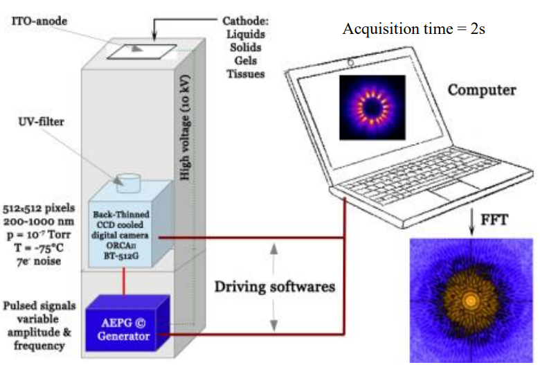
The device (see Figure 1) is composed of an AEPG© (Advanced ElectroPhotonic Generator), an EFUSE© (Electrode For Use in Specific Electrophotonic) electrode plate and a Hamamatsu HD camera (ORCA IIBT 512G2) coupled to an optic equipped with a UV filter (250-380 nm). The AEPG© is based on a particular geometry of its power transformers. Coupled with other components controlled by very reliable electronics, it produces, with its strong pulse voltage, an electromagnetic field on the electrode plate. This field is alternately positive and negative, with a predefined frequency selected on 90 Hz in this study. The frequency and voltage of the electromagnetic field are controlled by Advanced ElectroPhotonic Generator©, a self-developed software that also allows synchronization with the Hamamatsu camera. This field successively mobilizes electric charges on the surface and in the thickness of the object to be analyzed, causing the ionization of the gaseous environment around the studied body (plasma gas). This ionization creates an electron avalanche which, by splitting the gas molecules, releases UV photons that are recorded by the Hamamatsu camera. The electron avalanche then leads to filamentary structures called streamers (Chirokov et al., 2004; Kunhardt and Tzeng, 1998). Image acquisition provides an idea of the statistical distribution of light emission during exposure time.
Materials and Methods
Experimental Approach
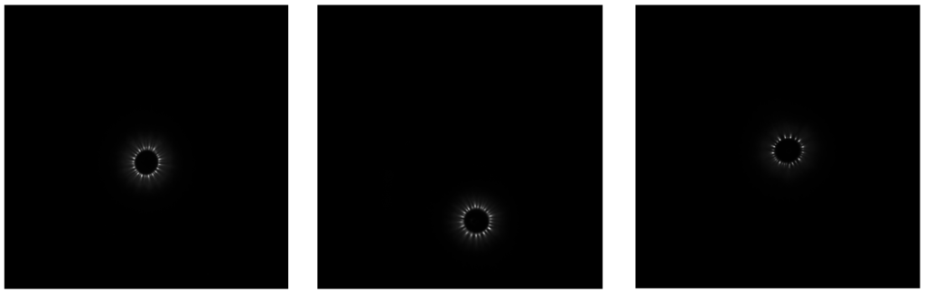
For each type of water selected, seven samples of the same water were collected. Ethanol is added to each sample to create a solution with an ethanol concentration of 1g/L to stabilize the phenomenon (we have found experimentally that ethanol allows better reproducibility and improved regularity of the corona shape). For each of these samples, ten 20 𝜇𝐿 droplets were stimulated, imaged, and analyzed. A specially designed pipette holder is used to reduce the background intensity on the images and to prevent stray light. A conductive nozzle is used on the pipette to deposit the droplet on the conductive, transparent electrode and stimulates it at a frequency of 90 Hz and a voltage of 11 kV for 2000 ms. The EDS© device then stores images in 16-Bits TIFF format of the corona discharge generated around the droplet. A database of 70 images (some examples are presented in Figure 2) for each kind of water is thus obtained.
The study will consist of studying and attempting to classify water types two by two. These water types are sugary water and salty water, then Native bottled water and Montcalm bottled water, then two river waters, from the Ariège and Garonne rivers.
Statistical Analysis
Parameter selection
The statistical analysis combines several methods that all start with the extraction of different parameters (see Appendix) from the images, such as the mean, the standard deviation, and the entropy, among a total of 86 final parameters (30 for the salty/sugary waters study) that characterize the corona, the streamers or the shapes found in the Fast Fourier Transform of the image. A class parameter is also defined to identify the groups (respectively 0 for salty, Montcalm and Ariège waters, 1 for sugary, Native and Garonne waters in the different studies). The other parameters are separated into numerical and categorical parameters and then sorted using between each parameter and the class parameter, the Pearson’s chi-squared statistic (Pearson, 1900) for the categorical parameters and the Pearson product-moment correlation coefficient (Pearson, 1895) for the numerical parameters. The retained parameters are those that are correlated with the parameter class with a p-value < 0.05. In parallel, the dataset, except for the class parameters, is normalized and analyzed by the Lasso model (Robert, 1994) to retain, in another way, the significant parameters. Among those retained, if two or more parameters are correlated with each other (defined by a Pearson’s r value > 0.8; Pearson, 1895), only the one with the highest correlation with the class parameter is retained. The method thus selects a set of significant parameters (whose number depends on the study) that will be used for the classification.
Classifiers
The resulting data are studied by five different classifiers among which is the KNN (K-Nearest Neighbors) classifier (Cover and Hart, 1967), which searches for the class of k neighbors in an x-dimensional space with x the number of selected parameters and k the number of neighbors chosen for classification. The naive Bayes Classifier assumes a conditional independence assumption (Chan et al., 1979) and it uses Bayes theorem (Bayes, 1763). The algorithm works by calculating the probability that a given data point belongs to each class, based on the features of the data point and the probabilities of membership of each feature to each class. The class with the highest probability is then chosen as the prediction. The other three classifiers operate with random hyper-parameters; these are the random forest classifier (Breiman, 2001), the decision tree classifier (Quinlan, 1986), and the gradient boost classifier (Freidman, 2001). Hyper-parameters are the adjustment parameters of the various Machine Learning algorithms (support vector machine [SVM], random forest, regression, gradient boost, etc). They differ according to the algorithm used. The best way to think of hyper-parameters is as the parameters of an algorithm that can be adjusted to optimize performance, just as we might turn the knobs on an FM radio to get a clear signal. For example, if we use random forest, we have the n-estimator as a hyper-parameter. This is a hyper-parameter that defines the number of trees to be used in our machine learning model.
The decision tree classifier is a supervised learning algorithm that works by constructing a tree-like model of decisions based on the features of the data. At each internal node of the tree, the algorithm splits the data based on a feature value, and the resulting splits are called “leaves.” Each leaf represents a decision based on the features of the data, and the final prediction is made by traversing the tree from the root to a leaf. The random forest classifier works by training multiple decision trees on random subsets of the training data and aggregating the predictions of those trees to make a final prediction. The gradient boost classifier is an iterative process in which a model is trained to predict the residuals errors of a previous model, and then the predictions of the current model are added to the predictions of the previous model to improve the overall accuracy. This process is repeated until a predetermined number of models have been trained, or until the error of the model has reached a certain threshold. For each of these classifiers, a cross-validation is performed with a stratified K-Folds cross-validator with k=8. Cross Validation is a technique for evaluating a machine learning model and testing its performance. One of the popular ways of doing a K-fold cross validation is to randomly shuffle the total data set and then divide the data set into K mutually exclusive identically sized subsets. Train on K-1 of these subsets and test on the Kth subset. Then go round-robin, K times. Train on another K-1 of these subsets and test on the Kth subset. Each time the tested Kth subset is different. The classification accuracy is then the average of all the K tests. The average of the AUC (Area Under Curve) (Narkhede, 2018) results for each classifier is then used to compare them. If one of the three classifiers with hyper-parameters is the best or the second-best classifier, an algorithm is used to try a combination of many hyper-parameters and retain the best combination of them. The classification results are the results given by the best and second best of the 5 classifiers after hyper-parameter optimization.
Experimental Results
Differentiation Between Salty Water and Sugary Water
Two solutions were prepared from salt (Guérande sea salt) and sugar (organic cane sugar). They were chemically very different to easily differentiate aqueous solutions during these initial trials. For this experiment, salty and sugary water samples were prepared from demineralized water with a salt and sugar concentration of 5g/L and an ethanol concentration of 1g/L. Droplets of those samples were then stimulated, imaged, and analyzed successively at different ambient air temperature and hygrometry (17.0±0.8°C, 63.6±2.4% of humidity for sugary water and 20.73±0.13°C, 54.02±0.47% of humidity for salty water). For this first experiment, 30 parameters were computed for each image. The Lasso method retains 6 parameters and the correlation with class method retains 17 parameters, including the 6 of the Lasso method. Three of the 17 selected parameters were highly correlated with some other selected parameters and were therefore excluded. The 14 resulting parameters are std, richness, h1, HS_value, meanStream, coronaLength, firstHalfLife, nbStreamer, frequAngStreamer, firstDecay, ampl2Pic, biodiv, diff1ersPics and HS_dist. For each of the 5 classifiers, an 8-splits K-Fold cross-validation is done and the results are shown in Figure 3.
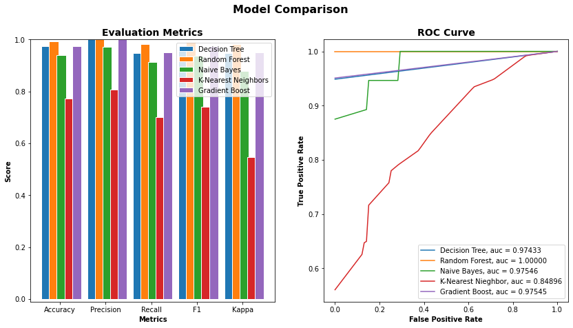
The two best classifiers based on the AUC are the random forest with an AUC = 1.0000 and the naive Bayes with an AUC = 0.97546. The random forest classifiers use hyper-parameters that would be optimized to get the final classifiers. Once the best hyper-parameters are computed, an 8-splits K-Fold cross-validation is applied on the resulting classifier to strengthen the results, and the naive Bayes is kept as it is (Figures 4a and 4b).
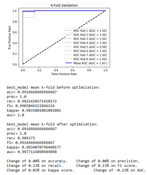
The results obtained between each cross-correlation vary little. It means that the model is reliable and predicts the right result almost systematically and it allows us to differentiate a salty water at 5g/L from a sugary water at 5g/L with an accuracy of 99%. The classification can be visualized in Figure 5. In this experiment, for each of the 17 significant parameters (the 14 used + the 3 highly correlated to at least one other significant parameter), every 2-D graphic can be shown to visually observe the classification. In Figure 5, the 2-D graphics can be seen for 7 of the 17 parameters that are arranged from top to bottom: angular frequency of the streamers (frequAngStream), mean of the streamers (meanStream), first decrease (firstDecay), second peak amplitude (ampl2Pic), length of the corona (coronaLength), standard deviation of the image (std) and Simpson’s Biodiversity Index applied on the image (biodiv).
Differentiation Between Montcalm and Native Bottled Water
The aim of this study was to try and differentiate between two chemically similar waters in plastic bottles. To do so, this experiment was carried out with Montcalm water and Native water since they are both low-mineralized waters. For this experiment, samples were collected from bottles of each water that were stored in the same room for several hours to equalize the temperature. Ethanol was added to obtain a concentration of 1g/L. They were then stimulated, imaged, and analyzed successively at the same ambient air temperature and hygrometry (17.15±0.46°C and 68.67±0.82% of relative humidity). With the 30 calculated parameters, the classification results were not very accurate; therefore, 56 new parameters were calculated for each image and added to the data. On the 86 parameters computed for each image, the correlation with class method retains 18 parameters (std, richness, l1, firstDecay, ampl1Pic, meanRatioSlopeMean, medianRatioSlopeMean, correlationStd, ratioSumEntropyCircle, meanRatioSlopeHigh10, medianRatioSlopeHigh10, ampl2Pic, varRatioSlopeMean, sumEntropyCircle, halfHighratioHigh10, entropyRatio, varHSCSdist, secondHalfLife) and the Lasso method retains 5 (richness, l1, nbCorrelInf75, nbCorrelInf50, nbCorrelSup95) of which 3 are already retained, keeping 21 parameters altogether (richness, l1, nbCorrelInf75, nbCorrelInf50, nbCorrelSup95, std, firstDecay, ampl1Pic, meanRatioSlopeMean, medianRatioSlopeMean, ratioSumEntropyCircle, meanRatioSlopeHigh10, medianRatioSlopeHigh10, ampl2Pic, varRatioSlopeMean, sumEntropyCircle, halfHighratioHigh10, entropyRatio, varHSCSdist,secondHalfLife). For each of the 5 classifiers, an 8-splits K-Fold cross-validation is realized, and the results are shown in Figure 6.
The two best classifiers based on the AUC are, like the first experiment, the random forest with an AUC = 0.98184 and the naive Bayes with an AUC = 0.97109. The best hyper-parameters for the random forest are computed, an 8-splits K-Fold cross-validation is applied on the resulting classifier to strengthen the results, and the naive Bayes is kept as it is (Figures 7a and 7b).
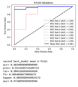
The obtained results lead to a slight decrease in nearly all the metrics for a very little increase of the AUC for the random forest. The naive Bayes, without hyper-parameters, remains the same. Those algorithms allow the technology to classify the water samples of Native and Montcalm with more than 92% accuracy with a good reliability.
In this experiment, for each of the 21 significant parameters (the 21 used + the 1 highly correlated to at least one other significant parameter), every 2-D graphic allows us to visually observe the classification. Figure 8 shows the 2-D distribution graphic for 7 of the 17 parameters that are arranged from top to bottom: standard deviation of the image (std), richness of the image (richness), L1-norm (l1), first decrease (firstDecay), first peak amplitude (ampl1Pic), mean of the ratios of the mean slope (meanRatioSlopeMean) and median of the ratios of the mean slope (medianRatioSlopeMean).
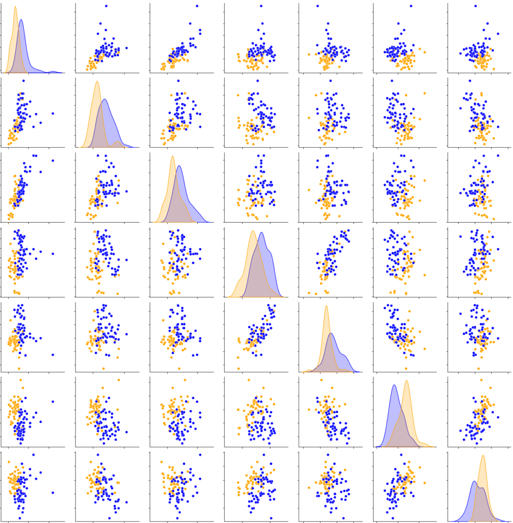
medianRatioSlopeMean for Native and Montcalm water.
Differentiation Between Ariège Water and Garonne Water
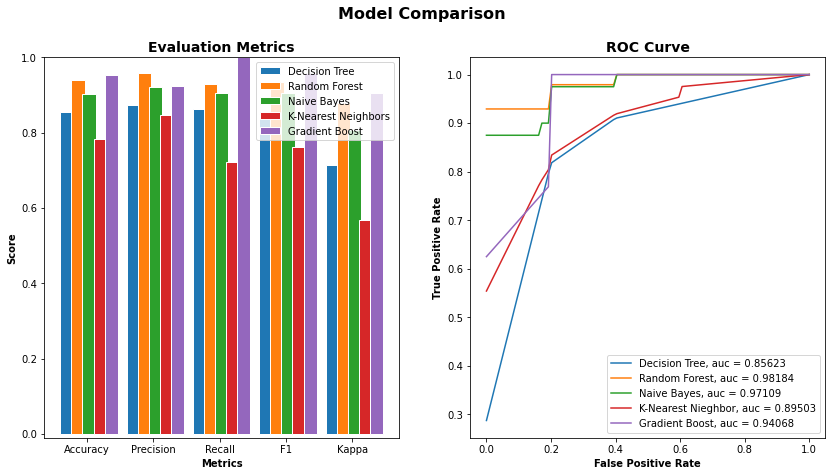
This experiment was carried out with waters from Ariège and Garonne, which are the two main rivers closest to the laboratory. The aim was to show that the technology could allow the differentiation between natural waters with potential applications in the environmental field. For this experiment, samples were collected from one location in each river, then stored in the same room for several hours to equalize the temperature. They were then stimulated, imaged, and analyzed successively at the same ambient air temperature and hygrometry (26.73±0.11°C and 50.97±1.08% of relative humidity). Of the 86 parameters computed for each image, the correlation with class method retains 26 parameters and the Lasso method retains 6 of which 3 are already retained, keeping 29 parameters altogether (mean, variance, stdLineMean, richness, nbCorrelInf75, nbCorrelSup95, nbDeperd95, firstDecay, ampl1Pic, diff1ersPics, stdRatioSlopeMean, medianRatioSlopeHigh10, correlationMean, meanRatiosZones30, stdRatiosZones45, ampl2Pic, meanRatioSlopeMean, medianRatioSlopeMean, ratioSumEntropyCircle, medianRatioSlopeHS, varCSHSdist, meanHSCSdist, hs_ValHS, meanRatioSlopeHS, halfHighICratioHS, firstHalfLife, secondHalfLife, nbStreamer, distance1stDecay). For each of the 5 classifiers, an 8-splits K-Fold cross-validation is done and the results are shown in Figure 9.
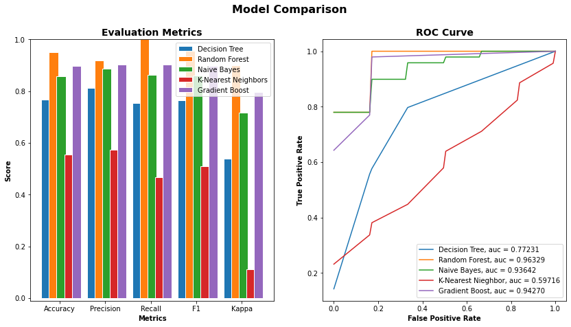
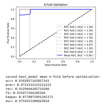
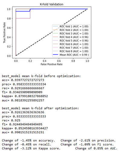
The two best classifiers based on the AUC are the random forest with an AUC = 0.96329 and the gradient boost with an AUC = 0.94270. Both of those classifiers use hyper-parameters that would be optimized to get the final classifiers. Once the best hyper-parameters are computed, an 8-splits K-Fold cross-validation is applied on the resulting classifier to strengthen the results (Figures 10a and 10b). The classification results can be viewed in Figure 11.
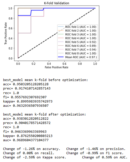
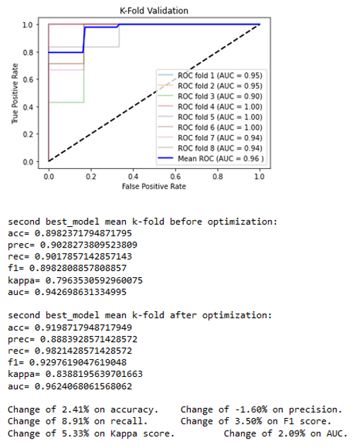
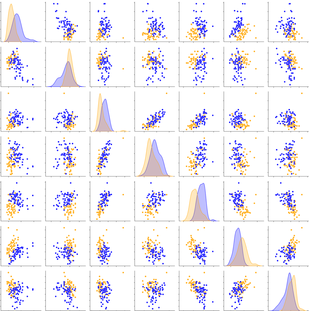
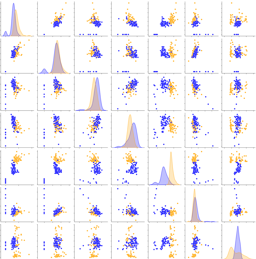
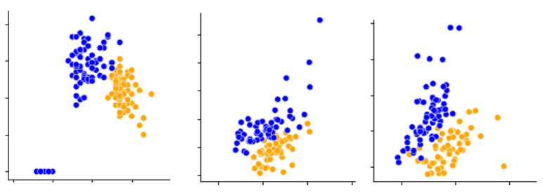
The obtained results lead to a slight decrease in nearly all the metrics for a very little increase of the AUC for the random forest and to a quite consequent increase in most of the metrics for the gradient boost. It allows the technology to classify the water sampled in Ariège and Garonne with nearly 94% accuracy with a good reliability. In this experiment, for each of the 29 significant parameters (the 28 used plus the 1 highly correlated to at least one other significant parameter), every 2-D graphic allows us to visually observe the classification. In Figure 11, the 2-D distribution graphics can be seen for 7 of the 17 parameters that are arranged from top to bottom: mean (mean), number of losses lower than 95% (nbDeperd95), first decrease (firstDecay), first peak amplitude (ampl1Pic), first peaks difference (diff1ersPics), standard deviation of the means of line (stdLineMean), and the standard deviation of the ratios of the mean slope (stdRatioSlopeMean).
Discussion
The most interesting results to emerge from this study are that CEMI technology combined with machine learning algorithms can differentiate between waters of different chemical composition. Although the computed parameters taken from the images and the classification methods can be reproduced with other electrophotonic devices, the results could be slightly different due to the specific conception of the EDS©. A new-generation, high-resolution scientific video camera that is more precise and can follow the evolution of the corona shape during capture, rather than taking a cumulative image and using stronger algorithms, should improve the quality of results. Except for room temperature and hygrometry, the room environment has not been monitored. The use of a clean room with controlled room parameters (air conditioned, absence of fine particles suspended in the air, and so on) and controlled electromagnetic interferences could produce more precise results but no such clean room was at our disposal. It would be interesting to add other measurement devices to go beyond classification and make it a tool to characterize water. Besides all those remarks, the results appear to be relevant to classify the different kinds of water using macroscopic corona imaging as shown by the algorithms results and Figure 12.
Conclusion
In this study, we used the specific device called EDS© to take UV-range pictures of corona discharges around droplets of water and we selected some parameters from these pictures to be used as predictor variables for a Data Science model. The aim of our study was to demonstrate the existence of a coherence between the photon energy fluxes generated during the irradiation of drops by EDS© and the physico-chemical properties of water, using a Data Science approach. The model is currently able to classify water types with an overall accuracy of more than 90%.
This suggests that the selected parameters and the machine learning models are effective at distinguishing between different types of water based on the images taken by the specific device. The ability to classify water in this way and the use of EDS© device to get information on liquids by a photonic method may have potential applications in a large variety of fields.
Concerning the measurements, we have a photonic tool that enables rapid (< 2 sec) and non-destructive capture, and a miniaturized tool that could be immersed in any environment. To quickly classify the waters tested using data science, we have constructed most of the 86 parameters used in this first approach. The list is not exhaustive. Our challenge was to show that, over a batch of captures, the photon fluxes captured during the corona effect are organized with a certain coherence linked to the product tested. We envisage industrial applications where this technology could be used as a “quality alert.” Before carrying out batteries of measurements on solutions to be controlled, we propose the possibility of monitoring the “photonic drift” of an in-process product in relation to an established situation. The monitoring and control of industrial processes is moving toward the use of big data. CEMI technology can rapidly provide large quantities of data. In the same way, we can imagine applications to identify counterfeit products from a few drops of liquid, for example, in wines and honeys, products with a high added value, and so on. More broadly, at a time when everyone is asking questions about the quality of natural waters and their evolution, we think it could be interesting to map the world’s waters with CEMI to observe variations. The data collected could be studied by researchers in a variety of ways (parameters, statistical tools, etc). It is possible to compare the CEMI with the microscope; on this basis, many applications are still to be discovered.
Acknowledgments
We would like to thank Eric Dombrowsky, one of the leaders of the Mercator Ocean project, for his support in developing this work on water using CEMI technology.
References
Arani R, Bono I, Giudice E, Preparata G (1995). QED coherence and the thermodynamics of water, International Journal of Modern Physics B (9) 15: 1813-1841.
Bayes T (1763). LII. An essay towards solving a problem in the doctrine of chances. By the late Rev. Mr. Bayes, FRS communicated by Mr. Price, in a letter to John Canton, AMFR S. Philosophical transactions of the Royal Society of London (53): 370-418.
Bono I, Del Giudice E, Gamberale L, Henry M (2012). Emergence of the coherent structure of liquid water. Water 4(3): 510-532.
Breiman L. (2001). Random forests. Machine learning 45: 5-32.
Carley JF, Kitze PT (1980). Corona‐discharge treatment of polymeric films, II: Chemical studies. Polymer Engineering & Science 20(5): 330-338.
Chan TF, Golub GH, LeVeque RJ. (1979). Updating Formulae and a Pairwise Algorithm for Computing Sample Variance. Department of Computer Science, Stanford CS tech report STAN-CS-79-773
Chen J, Davidson JH (2002). Ozone production in the positive DC corona discharge: Model and comparison to experiments. Plasma chemistry and plasma processing 22: 495-522
Chirokov A, Gutsol A, Fridman A, Sieber KD, Grace JM, Robinson KS (2004). Analysis of two-dimensional microdischarge distribution in dielectric-barrier discharges. Plasma Sources Science and Technology 13(4): 623.
Coudert FX (2007). L’eau et l’électron hydraté en milieu confiné : des propriétés physico-chimiques à la réactivité (Doctoral dissertation, Université Paris Sud-Paris XI).
Cover T, Hart P (1967). Nearest neighbor pattern classification. IEEE transactions on information theory 13(1): 21-27.
De Grotthuss CJT (1806). Sur la décomposition de l’eau et des corps qu’elle tient en dissolution à l’aide de l’électricité galvanique. Ann Chim 58: 54.
Einstein A (1905a). Does the inertia of a body depend upon its energy-content. Annalen der physik 18(13): 639-641.
Einstein A (1905b). On a heuristic point of view about the creation and conversion of light. Annalen der Physik 17(6): 132-148.
Fan J, Upadhye S, Worster A (2006). Understanding receiver operating characteristic (ROC) curves. Canadian Journal of Emergency Medicine, 8(1) 19-20.
Farzaneh M (1986). Contribution à l’étude des mécanismes des vibrations induites par effet de couronne (Doctoral dissertation, Toulouse 3).
Fresnel A (1826). Mémoire sur la diffraction de la lumière. Mémoires de l’Académie des Sciences V: 339-475.
Friedman JH (2001). Greedy function approximation: a gradient boosting machine. Annals of statistics: 1189-1232.
Hartmann G (1984). Theoretical evaluation of Peek’s law. IEEE Transactions on industry applications, 6: 1647-1651.
Henry M (2016). L’Eau et la physique quantique. Dangles, Escalquens.
Ignatov I, Mosin OV (2015). Non-equilibrium gas discharge conditions for origin of life and living matter. Experiments of Miller. Modeling of the conditions with gas coronal discharge simulating primary atmosphere. Journal of Medicine, Physiology and Biophysics 9: 27-50.
Janadri CS, Sheeparamatti BG, Kagawade V (2017, September). Multiclass classification of kirlian images using svm technique. In 2017 International Conference on Advances in Computing, Communications and Informatics (ICACCI): 2246-2250). IEEE.
Kononenko I (2001). Machine learning for medical diagnosis: history, state of the art and perspective. Artificial Intelligence in medicine 23(1): 89-109.
Korotkov K (2013). Energy fields electrophotonic analysis in humans and nature. eBookIt. Com: 68-77 and 100-140.
Kunhardt EE, Tzeng Y (1988). Development of an electron avalanche and its transition into streamers. Physical Review A 38(3): 1410.
Loeb L (1965). Electrical Coronas Their Basic Physical Mechanisms. University of California Press. ASIN B0006BM4LG
Maaroufi M (1989). Vibrations induites par effet de couronne. Université de Liège, France.
Malus EL (1811). Mémoire sur de nouveaux phénomènes d’optique. Journal de physique 72: 393-398.
Maxwell JC (1865). A dynamical theory of the electromagnetic field. Philosophical transactions of the Royal Society of London 155: 459-512.
McGraw-Hill (2007) Photocopying processes. McGraw-Hill Encyclopedia of Science and Technology 10th Edition, volume 13: 394-395.
Narkhede S (2018). Understanding AUC-ROC curve. Towards Data Science 26(1): 220-227.
Newton I (1952). Optics, or a treatise of the reflections, refractions, inflections & colours of light. Dover Publications Inc. New York, Book One: 1-193.Published in 1952 (based on the fourth Edition London, 1730).
Noll C. (2002). Ozone production by corona discharges. Journal of the IEST 45(1): 98-105.
Pearson K (1895). VII. Note on regression and inheritance in the case of two parents. Proceedings of the royal society of London 58(347-352): 240-242.
Pearson K (1900). X. On the criterion that a given system
of deviations from the probable in the case of a correla-ted system of variables is such that it can be reasonably supposed to have arisen from random sampling. The London, Edinburgh, and Dublin Philosophical Magazine and Journal of Science 50(302): 157-175.
Perakis F, Amann-Winkel K, Lehmkühler F, Sprung M, Mariedahl D, Sellberg JA, Nilsson A (2017). Diffusive dynamics during the high-to-low density transition in amorphous ice. Proceedings of the National Academy of Sciences 114(31): 8193-8198.
Planck M (1900). On the theory of the energy distribution law of the normal spectrum. Verh Deut Phys Ges 2(237): 237-245.
Pollack GH (2013). The fourth phase of water. Ebner and Sons Publishers: Seattle, WA, USA.
Quinlan J R (1986). Induction of decision trees. Machine learning 1: 81-106.
Robert T (1994). Regression shrinkage and selection via the lasso. Journal of the Royal Statistical Society Series B 58: 267.
Škarja M, Berden M, Jerman I. (1998). Influence of ionic composition of water on the corona discharge around water drops. Journal of Applied Physics 84(5): 2436-2442.
Tazuke S, Matoba T, Kimura H, Okada T (1980). A novel modification of polymer surfaces by photografting. ACS Symposium series 121, Modification of polymers, American Chemical Society, Washington D.C. 217-241
Vandanjon L (2021). L’interprétation quantique du rôle de l’eau dans le vivant, Ed. Matrix, ISSN 2266-9949, https://halo2mer.fr/dossiers/
Vieilledent G, Herren R, Morard V, Chaumet-Lagrange E (2016). EDS Electrophotonic DataPhoton System : une solution technologique innovante en imagerie macroscopique par effet de couronne. HEGEL, n°1(1): 3-9. Doi 10.4267/2042/58961
Voeikov V, Korotkov KG (2017). The Emerging Science of Water. CreateSpace Independent Publishing Platform.
Watterson JG (1987). A role for water in cell structure. Biochemical Journal 248(2): 615-617.
Wiggins P (2008). Life depends upon two kinds of water. PLoS One 3(1): e1406.
Young T (1802). II. The Bakerian Lecture. On the theory of light and colours. Philosophical transactions of the Royal Society of London 92: 12-48.
Appendix
Parameters:
As the process is patent pending, only a few parameters are detailed here. We’ll be able to provide interested scientists with further details following an NDA (No Diffusion Agreement) contract.
mean:
Average pixel intensity of the 260*260 image around the center of mass without background noise.
Mean = (Sum of all pixel values) / (Total number of pixels)
std:
Standard deviation of pixel intensity of the 260*260 image around the center of mass without background noise.
σ = sqrt((1/N) * Σ(xi – μ)²)
Where:
- N is the total number of pixels in the image (260 * 260 in your case).
- xi represents each pixel value in the image.
- μ is the mean value of the pixel intensities in the image.
- Σ represents the sum over all pixel values in the image.
variance:
Pixel intensity variance of the 260*260 image around the center of mass without background noise.
Variance = σ²
richness:
Number of sectors (number of different intensities) -1, given by the formula
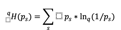
with ps the probability of obtaining each intensity and
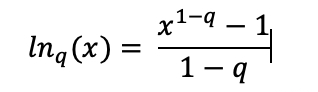 with q=0.
biodiv:
Simpson’s Biodiversity Index applied to the image. This is the probability that two pixels taken at random do not have the same intensity value. It is given by the formula
![]()
with ps the probability of obtaining each intensity and
![]() with q=2.
with q=2.
l1:
L1 norm is the sum of all pixel intensities.
where f(i,j) is the intensity of the pixel with coordinates i,j.
l2:
The L2 standard gives an idea of the total photon intensity and should remain roughly constant for similar materials. It is given by the formula
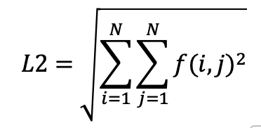 where f(i,j) is the intensity of the pixel with coordinates i,j.
FirstHalfLife:
On the Average Circular Intensity curve, this criterion measures the distance between the circle of highest intensity (the HotSpot) and the circle where intensity has been divided by 2. In other words, it measures the distance for intensity to halve from the HotSpot.
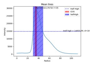
FirstHalfLife = dHsp/2 – dHsp
Where:
dHsp is the distance between the hotspot and the center of mass.
dHsp/2 is the distance between half of the hotspot value and the center of mass.
secondHalfLife:
On the Average Circular Intensity curve, this criterion corresponds to the distance required for the average circular intensity to drop from 50% of the HotSpot to 25% of the HotSpot.
SecondHalfLife = dHsp/4 – dHsp/2
Where:
dHsp/4 is the distance between one-quarter of the hotspot value and the center of mass.
dHsp/2 is the distance between half of the hotspot value and the center of mass.
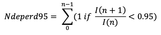
nbDeperd95:
On the Average Circular Intensity curve, we measure, from the hotspot, the ratio between the intensity at the distance n+1 and the intensity at the distance n. The parameter nbDeperd95 is the count of the occurrences when the ratio is inferior to 0.95.
Appendix Figure 1
h1:
The H1 standard provides a measure of the overall average contrast between all the pixels on the image. It is given by the formula:
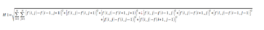 where f(i,j) is the intensity of the pixel with coordinates i,j.