
![]()
Study of Phase Coherence of Molecular Orientations in Coherence Domains of Water by Dynamic Molecular Simulation
JY Dolveck
Natur’Eau Quant Association, 187 Chemin du Mas Audibal, F-30360 VEZENOBRES
Keywords: Water, Molecular simulation dynamics, Coherence domains, Phase coherence
Published: March 21, 2021
Abstract
The properties of spatial phase coherence of molecular orientations in coherence domains in water are illustrated by dynamic molecular simulation. Nano-droplets of water are modeled. The behaviors of these nano-droplets in their ground state and in their excited state are compared through different models. Coherence of molecular orientations is studied in the presence or absence of a constant or alternating electric field in the microwaves range of frequencies. The input parameters are the intensity or the frequency of the field and the size of the nano-droplets. The output data studied are the cohesion energy, the electrostatic interaction energy with the electric field and the coherence degree of the molecular orientations. We then try to analyze and discuss the effect of the different types of molecular interactions on observed behavior of nano-droplets: it appears that non-oriented intermolecular interactions, such as London-type dispersive interactions for example, favor an increase in phase coherence of the molecular orientations unlike intermolecular electrostatic dipolar interactions.
Introduction
The hypothetical property of water, namely the existence of an excited state of the molecules in particular areas called “coherence domains” as a result of electromagnetic excitation, has been clearly described repeatedly by many scientists [1, 2, 3]. Experimental evidence of the existence of coherence domains has been reported by some laboratories under special conditions such as in molecular nanotubes [4]. The hypothesis that coherence domains might exist in other water environmental configurations [5] is also mentioned as a justification that water has a memory property.
It is assumed that the coherence domains can lie within biological cells [6, 7, 8] and that they possibly retain electromagnetic information emitted by the DNA [9] or various proteins. These electromagnetic waves can reveal pathogenic states of DNA damaged by oxidation. The detection of the electromagnetic signals is strongly correlated with the observations of polymerase chain reactions (PCR). For example, we can detect the infections with HIV or Lyme disease using this approach.
The characteristics of the coherence domains have been exhaustively studied [10]. There is a relationship of periodicity between the dimension of the excited zones and the wavelength of the corresponding energy gap. As the energetic gap is equal to 12.07 eV, the corresponding electromagnetic wavelength is equal to 75 nanometers, knowing the refractive index is 1.33 in liquid water. The periodicity of the coherence domains corresponds, in fact, to this wavelength. The excited water molecules are in the energy potential maxima and the ground state molecules are in the energy potential minima. Thus, the description of this phenomenon implies the existence of a trapped photon. Some authors have shown through spectroscopic methods such as microwave or near infrared spectroscopy that the presence of the coherence domains leads to characteristic spectra which evidence the existence of two energetic states of water [11, 12].
The excited water molecules may have coherent orientations in the coherence domains, particularly in the presence of an electromagnetic field. The consequence is a greater sensitivity to the electromagnetic fields. Conversely, ground-state water molecules may be much less structured. This coherence of molecular orientations concerns several million molecules in a coherence domain. It is therefore difficult to reproduce this phenomenon in a whole coherence domain, particularly by dynamic molecular simulation because of the computing power required.
The present work will therefore only illustrate this property of coherence of the orientations in small environments, such as nano-droplets of water molecules, with the dynamic molecular simulations [13]. According to the literature, the nano-droplets of water have been in fact the object of several studies by dynamic molecular simulation in various environments such as carbon nanotubes, zeolites or copper surfaces [14, 15, 16] and these studies allowed to evidence particular water structures. In the present study, an electric field is used in order to stimulate the nano-droplets. This electric field may be constant or alternating with a variable amplitude or frequency. Three molecular models will be studied: a “fundamental” model of water molecules in their ground state and two models of molecules in their excited state as in the coherence domains. The first model of the excited state, called the “intermediate” model, will take into account the dipolar interactions (so called Keesom interactions [17]) between the molecules in a less important part and London-type dispersive interactions [18] in a significant part. The second model of the excited state, called the “forced” model, will consider that the intermolecular dipolar interactions do not exist and that they are entirely replaced by strong dispersive London-type interactions. These last two models are justified by the existence of an almost free and highly mobile electron in the non-binding orbitals of the oxygen atom of excited water molecules. Thus, the oxygen atom can become highly polarizable.
This choice of an environment such as nano-droplets does not presume to illustrate a real experimental or natural context but it is used to simplify the approach. One supposes here the quantic states of the water molecules, fundamental or coherent, are stable in the nano-droplets. Obviously, it is an approximation of reality and it may be justified by the short durations of the simulation runs. In their excited state, the water molecules are still considered as independent entities like in their fundamental state. This assumption is probably not exact, but it will allow a comparison with a total quantic approach supported by ab initio simulations.
We will try to analyze the relationship between the phase coherence property of the orientations of the molecules and the energy properties of the coherence domains thus simulated by comparing these properties to those of the nano-droplets of water in their ground state, in interaction with the electric field. We will seek to determine the effect of the intensity of the electric field, and the effect of the frequency in the case of an alternating electric field, and also the influence of the intermolecular interactions on the coherence of the orientations of the molecules, through the comparison of the different models. We will notably try to compare the results obtained with a modeling of the evolution of energy properties with frequency. The used frequencies will be in the domain of microwaves around the absorption frequency of water (about 20 GHz at 20°C) [19].
Bibliographic Data and Theoretical Framework
Water in its fundamental state: Some physical properties of liquid water are indicated in Table 1: the molecular weight M, the boiling temperature Tb, the enthalpy of boiling ΔΗb, the liquid heat capacity Cpl and D density at 20 ºC [20].
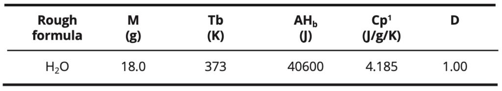
Table 1. Some physical properties of liquid water in its fundamental state.
The enthalpy of boiling and the high boiling point of water, relative to its low molecular weight, are due to the strong dipolar interactions between the molecules. These interactions are modeled by hydrogen bonds. These are numerous in liquid water. In comparison, methane, which has almost the same molecular weight (16 g) but only involves the weak intermolecular London-type interactions, has a low boiling point (-161 °C) and a low boiling enthalpy. On the other hand, other compounds such as ammonia or hydrogen fluoride, which also involve hydrogen bonds, have a lower boiling point and a lower boiling enthalpy too.
The water has a high relative dielectric constant (εr = 80). This is related to the high dipole moment of the water molecule: μ = 1.85 Debye. Water has a very low conductivity due to its low dissociation equilibrium constant (Ke = 1E-14) in the pure state. The presence of dissolved ionic species can greatly increase its conductivity.
Coherence domains [1, 2, 3, 10]: In many studies, it has been shown that collections of water molecules can have excited states under certain conditions. These excited states are called “coherence domains.” They are particularly characterized by the indiscernibility of the molecules which behave as a single entity. The explanation of this phenomenon involves quantum physics. The excited state is due to an energy transition of an electron located in the non-binding electronic orbitals of the oxygen atom. This electron goes from the 2p orbital to a 5d orbital and may be less bound to the oxygen atom. The corresponding energy gap has a height of 12.07 eV and is linked to a photon whose wavelength is equal to:
(1) λ = c / ν = c h / E
According to the relation: E = h ν (and then ν = E / h)
Where:
c is the celerity of light: c=3E8 m / s
h is the Planck constant : h = 6.62E-34 J.s = 4.13E-15 eV.s
λ is the wavelength of the photon in meters
ν is the wave frequency in hertz
The corresponding photon to the electromagnetic field associated with the coherence domain is trapped in a quantum box resulting from a grouping of the excited molecules. The periodicity of the clusters is then equal to the wavelength of the trapped photon. According to the frequency of the photons f = 3E15 Hertz which corresponds to the energy gap of 12.07 eV and the index of refraction in water n = 1.33, the periodicity of the coherence domains thus measures 7.5E-8 m or 75 nm. This approach is explained in Figure 1.
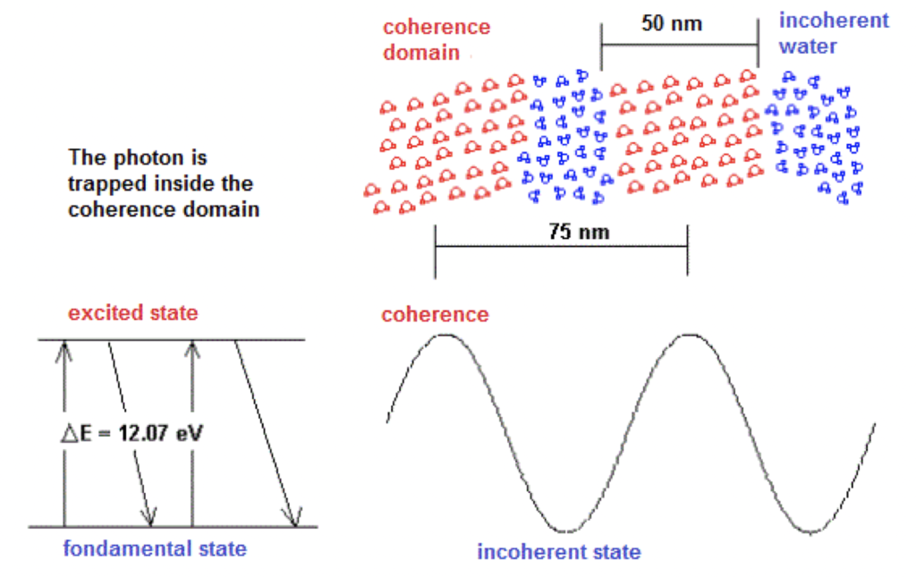
Figure 1. Structure of the coherence domains in water.
The electromagnetic waves associated with the coherence domains are stationary. The phase speed is much higher than the group speed. At the time scale of the laboratory, the rate of fluctuation of the coherence domains is very high but it is much lower than the frequency of the electromagnetic wave. The coherence domains form a three-dimensional fluctuating structure. A spherical coherence domain of 50 nm in diameter would contain about 4 million molecules. Water molecules have a very slow rate of displacement at room temperature compared to the fluctuation of coherence domains. Thus, the oscillation between the ground state and the excited state of the molecules takes place like the mechanism of the Mexican wave: the molecules gradually reach the state of excitation and fall in a similar way until the ground state.
Coherence of molecular orientation: One of the properties of coherence domains, related to the indiscernibility of molecules, is the coherence of the molecular orientations. It is observed that the electric dipoles formed by the water molecules in their ground state have various orientations in time and in space due to thermal agitation. In the coherence domains, the orientations of the molecules should be better organized spatially at room temperature. This property is related to a high sensitivity of coherence domains to electromagnetic fields. A pictorial way of describing a coherence domain is the comparison with a school of fish. This coherence of orientations is dynamic and the global orientation of the molecules can fluctuate over time, but the dispersion of the molecular orientations is very weak.
If we consider two electric dipoles d1 and d2, we can evaluate the dispersion angle of their orientations in space as follows, described in Figure 2. The vector S results in the average sum of the dipole modules and the vector M is the average sum of the dipolar vectors of each dipole. The ratio d = M / S characterizes the degree of coherence and the dispersion angle θ is then calculated as follows:
(2) θ = 2 * arcos (M / S)
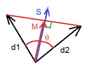
Figure 2. Phase dispersion measurement.
This method of calculation can be generalized to a group of dipoles and a mean degree of spatial phase coherence and a mean dispersion angle are obtained.
Settings of Molecular Dynamic Simulation
For the more complete details one may refer to the annex. However, the principal lines of the simulation processing are explained as follows:
Computer Software: Molecular dynamics simulations are performed on a personal computer with a personal Java program. A Monte Carlo algorithm is used to move each atom or electron doublet in the simulated molecules. The energy potential is calculated both in the initial position and in the end position of the moved entity. If the difference is negative, the move is always allowed. If it is positive, the displacement of the entity depends on a probability threshold Pt of displacement according to the Boltzmann relation:
(3) Pt = exp [-(Uf – Ui) / k T]
Where:
Ui and Uf are the initial and final energetic potentials.
T is the temperature in Kelvins.
k is the Boltzmann constant.
A random variable is called. If it is less than Pt, the move is allowed. In the other case, it is forbidden. The length step for the calculation of the potentials is equal to 0.005 nm. After each sequence of 100 computation loops in which all the entities are moved, the program gives an updated image of the system. This will be chosen as the unit of time in the simulations and corresponds approximately to a real time of 0.2 picoseconds.
Molecular modeling: The water molecule is simulated both in its ground state and in its excited state, using some models involving five entities: the oxygen atom, the two hydrogen atoms and the two electronic free doublets. This approach resembles a Ti5P water model [21]. In the excited state of the molecule, the free electronic orbitals are larger and their distance to the oxygen nucleus is longer than in the ground state. The van der Waals radius of the oxygen atom is also increased. The OH bond will however be the same in both types of models and is here equal to 1.00 Å (or 0.100 nm). The Van der Waals radius of hydrogen is equal to 1.20 Å (or 0.120 nm) in both cases. Table 2 explains the different parameters.
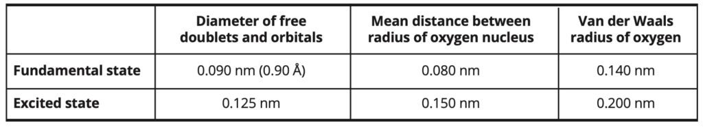
Table 2. Parameters and dimensions of water molecules.
The intramolecular and intermolecular interactions involved in the simulations are exposed in Table 3.
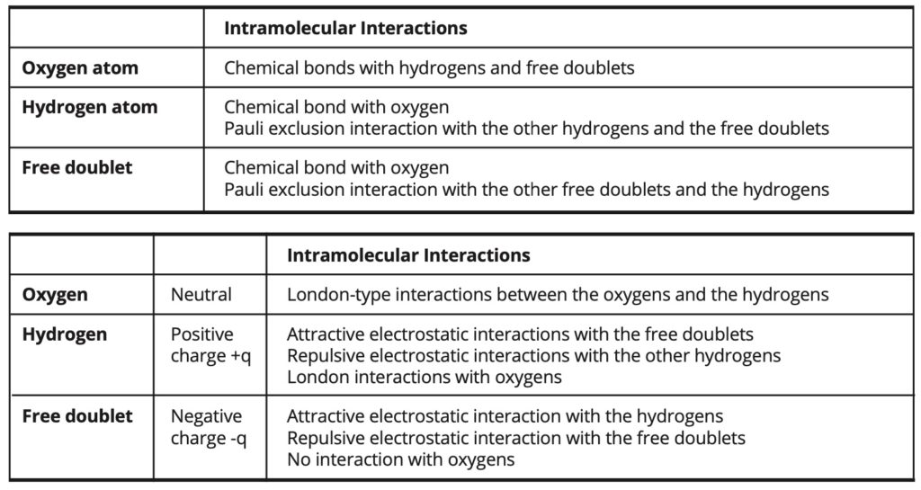
Table 3. Intramolecular and intermolecular interactions.
In the case of the intermediate model, the intermolecular electrostatic interactions are weaker than in the fundamental model and they are partially replaced by some London- type interactions of greater intensity. In this case, the electrostatic portion of the cohesion energy amounts to 72% of the total cohesion energy, whereas it amounts to about 100% of the cohesion energy in the fundamental model.
In the case of the forced model, the intermolecular electrostatic interactions are entirely replaced by London-type interactions, which are then of greater intensity than in the intermediate model.
• The chemical bond potentials are parabolic with a minimum energy level at the average bond length.
• Pauli’s exclusion interactions are parabolic and vanish when the distance between the centers of the atoms is greater than the Van der Waals distance.
• The London-type interactions are represented by the Lennard-Jones type potentials [22] with a minimum of the energy level at a distance equal to the sum of the van der Waals radii of the interacting atoms.
• Attractive and repulsive electrostatic interactions are represented by Coulomb potentials.
Modeling of the electric field: The electric field is constant or alternating sinusoidal. It has a constant direction on the y-axis. The periodic function that describes the alternate field has the following form:
(4) E(t) = Em sin(2 π f t)
Where: Em is the amplitude and f is the frequency.
The electric potential is described in all the space by the following function:
(5) V(t, y) = y E (t) + Vo
It is constant in Ox and Oz directions. The constant Vo is chosen equal to zero at y = 0.
The energetic potential of an electric charge q (proton or electronic free doublet) in the electric field has got the following expression:
(6) Uq(t) = q V(t, y) = q y E(t, y)
This leads in particular to the expression of the electric energy of a water molecule in the electric field:
(7) Um(t) = 2 q E(t) d cos(α)
α is the angle between the direction of the molecular dipole axis and the orientation of the electric field and d is the dipole distance. For the water molecules in their ground state, d = 0.060 nm. This value may be slightly different in the simulation because of the various approximations in the modeling.
In the used molecular models, fundamental state or excited state, the electric charges on the hydrogens and on the free doublets are in fact adjusted in order to have for one insulated molecule the same interaction energy in the same intensive electric field in these two quantic states.
The simulated intensities of the electric field vary from 2500 to 10 000. These values are expressed in arbitrary units. In the case of an intensity E = 10000, the electrical energy per molecule represents about 20% of the cohesion energy per molecule in liquid water. The corresponding real intensities of the electric fields range approximatively from 1E9 to 4E9 V/m. These high values are therefore inferior to the dipolar electric field which is more than 1E10 V/m close to the water molecule (It then corresponds to simulated field intensities greater than 25000) at a distance inferior to 0.3 nm (which is the average distance between the mass centers of the water molecules in the liquid state).
The simulated frequencies of the alternating electric field range from 1E-4 image ^ -1 to 1 image ^ -1. In comparison, the relaxation frequency of the simulated water molecule in its ground state is about 3E-3 image ^ -1 and corresponds to 20 GHz, which is the relaxation frequency of the real water molecules. Then, the simulated frequencies correspond to the range of 600 MHz to 6 THz. Thus, the highest simulated frequencies (≥ 5E-2 image ^ -1) are located in the far infrared domain (≥ 300 GHz). The duration of a simulation run is here 10 000 images long. It then corresponds to a real duration of 1.5 ns. It is assumed that the quantic state of the water molecules is stable during this period.
Simulation of the nano-droplets of the water molecules: The simulated nano-droplets contain 8, 18 or 27 molecules. The density of water in its fundamental state is taken equal to 1.200. The density of water in its excited state is taken equal to 0.800. The mean density value is then equal to 1.000. The temperature is always equal to 20°C.
The elemental volume Ve occupied by a molecule is calculated as follows:
(8) Ve = VM / N = (M / D) / 6.02E23
Where VM is the molar volume, M the molecular weight, D the density and N the Avogadro number.
The simulation boxes are cubic and their dimensions are calculated according to the elementary free volume and the number of molecules in the nanodroplet.
Figure 3 illustrates the representation of the modeled water molecules in their ground state and in the excited state: the oxygen atoms are red, the hydrogen atoms are cyan. The electronic non-binding pairs are pink in color.

Figure 3. Representation of the simulated molecular models, fundamental: left, excited: right.
The acquisition will be made by averaging the simulation data on three runs for each simulation. A simulation run lasts 10000 pictures.
The cohesion energy of the nano-droplets, their interaction energy in the electric field and the degree of the spatial phase coherence are measured. The dispersion angle of the phase is deduced from Equation 2.
The unit used for Esim cohesion energy is arbitrary. The following correlation law (9) makes it possible to convert the values of the simulation into joules per mole of the considered entity. The entity is the nano-droplet, whatever its size.
(9) E (J / mol) = Esim / 26.7
Simulation Results
Cohesive energy: Graph 1 shows the evolution of the cohesive energy in the three simulated models: fundamental FS, intermediate: IM, and forced: FM. It illustrates either the evolution without electric field or in a constant high intensity electric field (E = 10000). Linear adjustments were also represented.
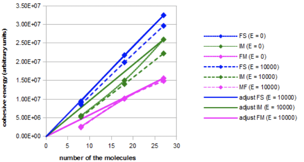
Graph 1. Evolution of the cohesive energy for the three models as a function of the nano-droplet size in absence (E=0) or in presence of a constant electric field (E=10000).
The total cohesion energy increases with the nano-droplets size. The increase is linear in the fundamental model, but not in the intermediate and forced models. The cohesive energies are not equal for the same nano-droplets size, but this result may not be related to the experimental reality because of the arbitrary choice of the parameterization of the London-type interactions. The cohesion energy decreases when an intense electric field is applied in the fundamental and intermediate models, but not in the forced model.
When the electric field is increasing, more complete simulations show that the decrease of the cohesion energy occurs more and more rapidly in the fundamental model and in the intermediate model. On the contrary, the cohesion energy does not decrease in the forced model.
Graph 2 shows, in the three simulated models (nano-droplets of 27 molecules), the evolution of the cohesion energy when an intense alternating electric field (Em = 10000) with variable frequency is applied.
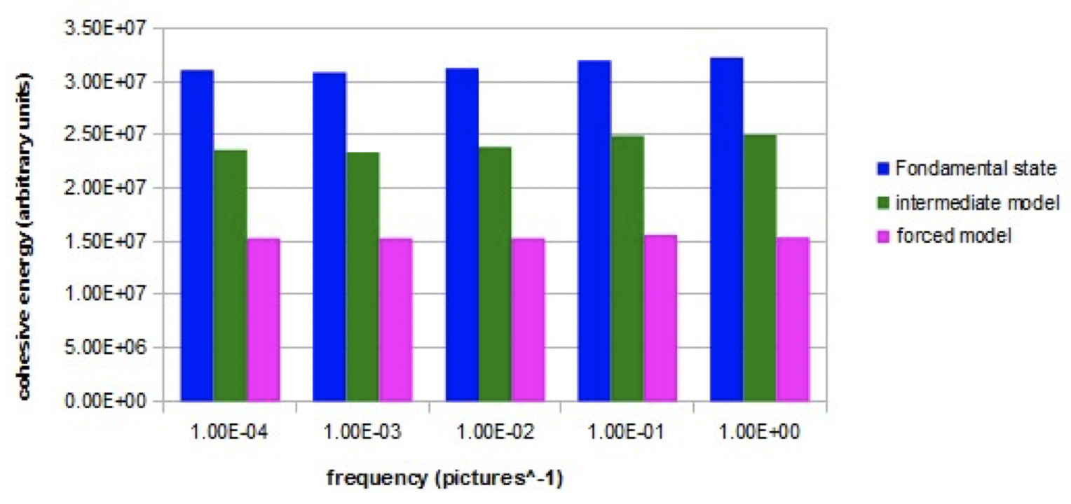
Graph 2. Evolution of the cohesive energy as a function of the frequency of the alternating electric field (E=10000) for the three models.
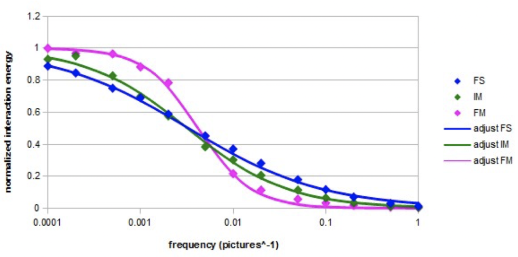
Graph 3. Normalized interaction energy of a nano-droplet containing 27 molecules as a function of the
frequency of the alternating electric field (Em=10000) for the three models.
For the fundamental model and the intermediate model, the cohesion energy is lower at low frequencies than at high frequencies. The increase is significant between 1E-3 and 1E-1 image ^ -1. For the fundamental model, this increase represents about 5% of the average cohesion energy. For the forced model, the cohesion energy is constant at all frequencies.
Energy of interaction with the electric field: In the three models, the interaction energy in a constant intense electric field (E = 10000) increases with the nano-droplets size. The interaction energy is the highest for the forced model and it is the lowest for the fundamental model.
In the fundamental model and the intermediate model, the variation of the interaction energy in the constant electric field is parabolic when the intensity of the field increases. In the forced model, the variation is not parabolic and approaches the linearity.
The normalized variation of the interaction energy in an intense alternating electric field (E = 10000) at the different frequencies is represented on the semi-logarithmic Graph 4 in the case of a nano-droplet of 27 molecules for the three models. The adjustments were made according to the following equation, which is a simplified form of Cole-Cole equation [23, 24]:
(10) U = Uo / (1 + (f / fo)β) β ≤ 2
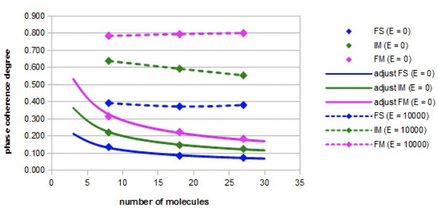
Graph 4. Evolution of the coherence degree with the number of molecules in the nano-droplets in presence (E = 10000) or no (E = 0) of a constant electric field.
The normalized interaction energy decreases as the frequency increases. The shape of the variation curve is sigmoidal. In the case of the three models, a cutoff frequency is observed. The cutoff frequencies are almost equal for the fundamental model and the intermediate model. In the case of the forced model, the cutoff frequency is slightly higher. The found values of the adjustment parameters fo and β are given in Table 4.
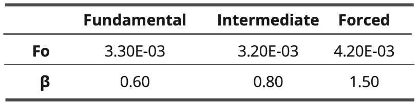
Table 4. values of adjustment parameters for the three models
The coefficient β has the lowest value in the fundamental model and it is the highest in the forced model. In the latter case, the relaxation almost resembles a simple Debye relaxation (characterized by β = 2).
Coherence degree of molecular orientations: The variations of the coherence degree of the molecular orientations as a function of the nano-droplet size in the absence of an electric field (E = 0) or in the presence of an intense constant electric field (E = 10000), are shown in Figure 4 for the three models: the fundamental model (FS), the intermediate model (IM), and the forced model (FM).
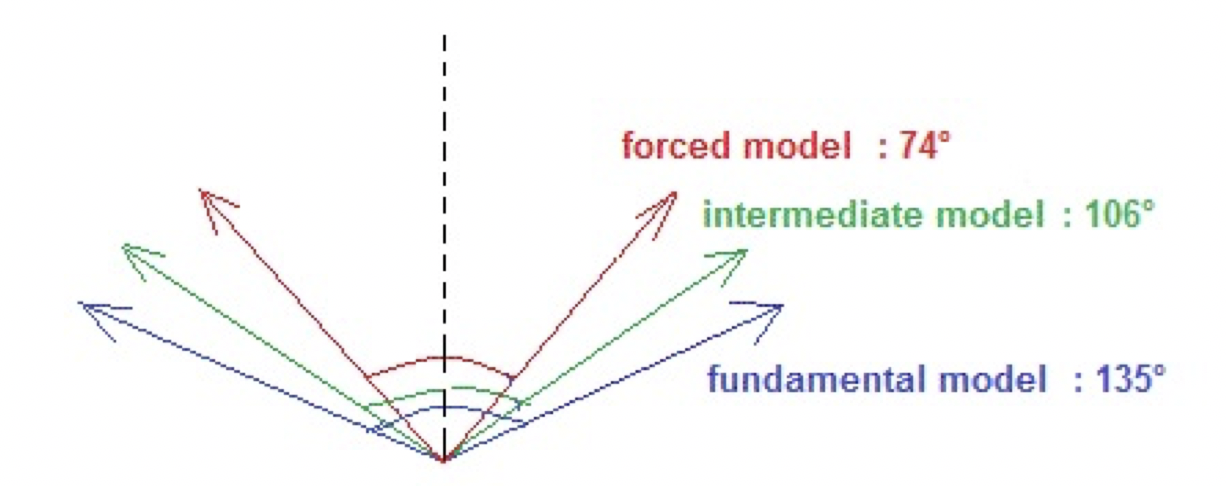
Figure 4. The dispersion angles in presence of a strong constant electric field (E = 10000) for a nano-droplet containing 18 molecules.
The coherence degree of molecular orientations is much higher in the presence of the electric field than when there is no electric field. When the electric field is applied, the coherence degree of orientations is the highest in the forced model and the lowest in the fundamental model. In these two extreme cases, the coherence degree is constant as the nano-droplet size increases. In the intermediate model, the degree of phase coherence decreases slightly as the nano-droplet size increases. In the absence of an electric field, the coherence degree decreases in all cases according to the inverse of the square root of the nano-droplet size. These adjustments are relatively accurate (the relative error is less than 4%).
Figure 4 illustrates the corresponding dispersion angles in the three models when a constant high intensity electric field (E = 10000) is applied.
Even if in the forced model, the angle of dispersion of the phase is the smallest, it is not close to the angle zero. Indeed, during the simulations, a fluctuation of the molecular orientations is observed.
Graph 5 shows the relative evolution of the coherence degree of the orientations (nano-droplet of 27 molecules) with the frequency of the electric field (intensity Em = 10000) in the three models.
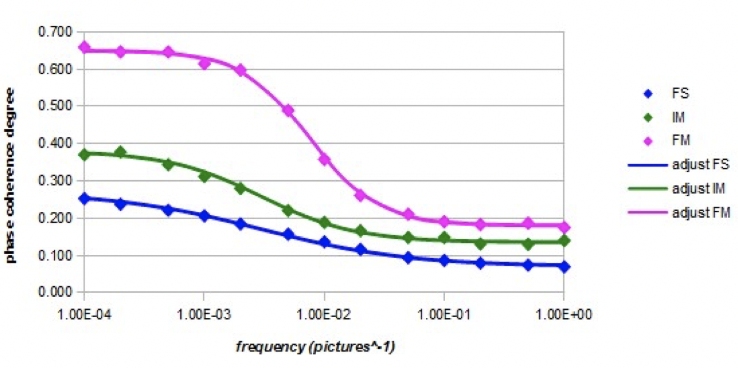
Graph 5. Evolution of the coherence degree as a function of the frequency of the alternating electric field (intensity Em = 10000) for the three models.
The three curves are sigmoidal with a cutoff frequency. The forced model has the highest cutoff frequency, while for the other two models the cutoff frequencies are lower and almost identical. Parameters fo and β are shown in Table 5 (adjustments by equation 10).
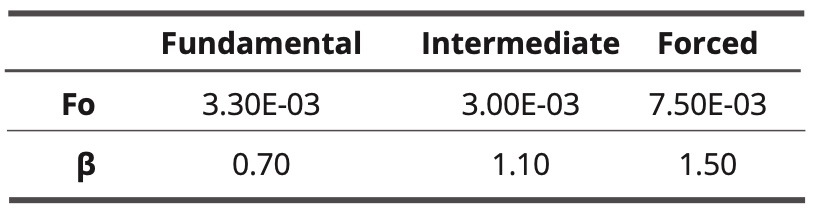
Table 5. Values of adjustment parameters for the three models.
The highest coefficient is the fit of the forced model curve, which almost characterizes a Debye-type relaxation.
In the forced model, the Figure 5 shows the images of a nano-droplet of eight molecules at different times during a period of oscillation of the electric field (Em = 10000, f = 1E-4 images).
The molecules globally change their orientations according to that of the electric field, but all the molecules are not rigorously oriented in the same direction.
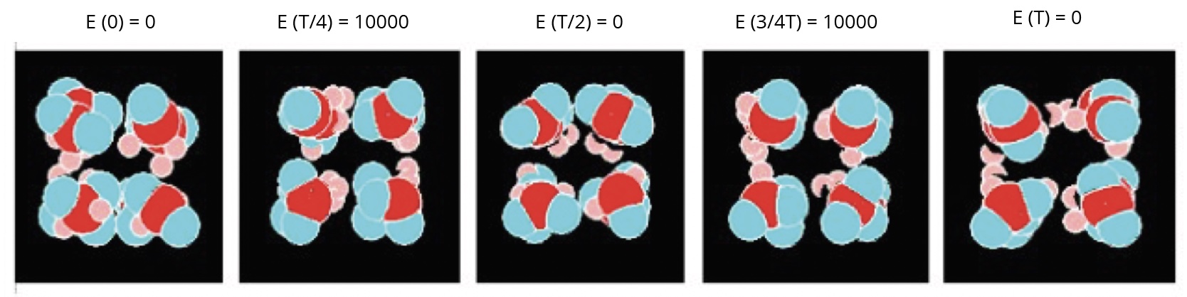
Figure 5. Different views of a nanodroplet of eight molecules in the alternating electric field.
Discussion
The three models have different behaviors. We will try to analyze the main factors that led to the previous results.
Behavior in the absence of an electric field: Graph 1 shows that the cohesion energy evolves differently for the three models. It increases linearly with the number of molecules in the nano-droplets only in the fundamental model where there are only intermolecular dipolar interactions. In the intermediate model and the forced model, where the dispersive intermolecular London-type interactions are present or preponderant, the linearity is not observed.
Graph 4 shows that the coherence degree of molecular orientations decreases with the square root of the number of molecules in the nano-droplets for the three models. Here we recognize a behavior in accordance with the normal law. Larger nano-droplet sizes could be usefully simulated to test whether this evolutionary law can be extended to a larger set of molecules. The forced model that uses only London-type intermolecular interactions leads to the highest values of the degree of spatial phase coherence. The fundamental model that involves only intermolecular dipolar interactions has the lowest values. Probably, dipolar interactions have a dissipative effect on the organization of molecules, which would not be the case for the London-type interactions. But we must also take into account the effects of small simulation boxes that can impose an organization of molecules, especially in the intermediate model and the forced model for which the oxygen atom of the water molecules is greater than in the ground state; Figure 5 shows that the molecules of small nano-droplets are arranged as a cubic form. This is not the case with the fundamental model where the van der Waals radius of the oxygen atom is smaller.
Behavior in the presence of a constant electric field: Graph 1 shows that the cohesion energy decreases in the presence of a constant electric field in the fundamental model and in the intermediate model, for which intermolecular dipolar interactions are present. We can assume the existence of an intensity threshold above which the cohesion energy becomes zero. But no linear behavior of these decreases has been observed during complementary simulations and so there is no possibility of accurate predictions. Some more intense electric fields should therefore be simulated. In the case of the forced model where only the London-type intermolecular interactions are present, there is no decrease in the cohesion energy. In the case of the forced model, The London-type intermolecular interactions are not disturbed by the electric field.
The coherence degree increases when the electric field is applied and this effect is much greater in the forced model than in the other models. But full simulations show that a saturation effect at the value of 0.80, so not 1.00, was observed for electric field intensities higher than 7500. The corresponding dispersion angle is then not equal to zero, as shown in Figure 4. The orientations of the molecules cannot be completely spatially synchronized. We cannot exclude a possible steric hindrance caused by the simulation boxes.
Behavior in the presence of an alternating electric field at variable frequencies: Graph 2 shows that the cohesion energy increases with the frequency of the alternating electric field in the fundamental model and the intermediate model, whereas in the forced model, the cohesion energy remains constant. At high frequencies, the cohesion energy is equal to that obtained in the absence of an electric field. In the fundamental model and in the intermediate model, a relaxation threshold can be highlighted and it is in the range 1E-3 to 1E-2 image ^ -1. It is probably related to the relaxation frequency of the simulated water molecules. At low frequencies with regard to the effect of the different types of intermolecular interactions, one can formulate the same conclusions as in the case of a constant electric field. At high frequency, the three models behave as if there was no electric field. In particular, in the case of the fundamental model and the intermediate model, because the molecules can no longer follow the orientation of the electric field, the latter no longer influences the intermolecular interactions.
Graph 3 shows that the interaction energy with the electric field also decreases with the frequency and that there is a relaxation threshold that may correspond to the relaxation frequency of the water molecules (4E-3 image^-1 here, which is equivalent to 20 GHz). In the three models, the decrease is total but it is more or less rapid around the relaxation frequency. In the case of the fundamental model and in the case of the intermediate model, we can invoke the contribution of dipolar interactions to explain the low values of the coefficient β (Table 4). In the case of the forced model, β is the highest, which makes it possible to conclude that the London-type dispersive interactions do not interfere with the reorientation movements of the dipoles and that they thus lead to less interdependent intermolecular behaviors, as in the case of a Debye-type relaxation [25].
Graph 5 shows that the coherence degree decreases significantly as the frequency increases. There is an effective correlation between the variations of the interaction energy with the electric field and the degree of phase coherence. At high frequencies, it is noted that the degree of phase coherence has a value equal to that obtained when there is no electric field. The relaxation frequency is higher in the case of the forced model than in the case of the other two models. This could be related to some possible inversions between the electronic-free doublets positions and the hydrogens positions in the molecule, since the mobility of the orbitals is greatly increased and their motion is also not hampered by dipolar intermolecular interactions which are not present in the forced model. In the case of the intermediate model, it is likely that intermolecular dipole interactions, which involve electrostatic interactions between non-binding electron pairs and hydrogen atoms, partially hinder this orbital inversion phenomenon.
Some correlations with experimental investigations: according to the author [11], Microwave spectroscopy analysis results carried out on water show some characteristic peaks which are associated with the presence of coherence domains that have a semi-crystalline structure. According to this work, the frequencies of the absorption peaks are higher than that of the rotation of the water molecules (20 GHz) and are around 50 GHz and then at a frequency 2.5 times higher. There is an analogy between these experimental results and those simulated in Graph 5 and Table 5 (about the coherence degree) in which the cut-off frequency of the coherent water simulated using the forced model (7.5E-3 image^-1) is 2.5 times higher than that of the water simulated in its fundamental state (3.0E-3 image-1). The simulated frequencies correspond here to 45-50 GHz and 18-20 GHz. According to the images of the simulations (Figure 5), the simulated coherent water would have a more ordered structure than simulated water in the ground state.
It would therefore be interesting to carry out simulations with a larger number of molecules to confirm these similarities in results on a larger scale. The small number of molecules involved here may illustrate with a relative fidelity the behavior of water molecules localized between the proteins in a biological environment. Some experimental investigations such as Coherent Raman Scattering Microscopy, which shows evidence that the water molecules are ordered near phospholipids layers, [26] may then confirm here the step of the present approach. In the case of a natural environment such as the waterfalls, one may consider that the droplets contain a much higher number of molecules and then the bounding effects would be neglected. It would be thus necessary to run the modeling with a much greater number of molecules and use the periodic conditions [13].
Conclusion
The present work consisted in simulating coherence domains in an excited state of water, in comparison with water in its ground state, involving the molecular dynamic simulation of some nano-droplets of water. Three models have been implemented: a “fundamental” model for water in its ground state and two models for water in an excited state: an “intermediate” model and a “forced” model. The intermediate model takes into account intermolecular dipolar interactions in a smaller proportion than in ground-state water, and a significant portion of London-type intermolecular interactions. The forced model involves only some intense London-type intermolecular interactions. The coherence degree of the molecular orientations has been characterized in particular by the coherence degree and the dispersion angle. We have also tried to highlight correlations on cohesion energy measurements and interactions with a constant or alternating electric field.
The principal results are the following:
• In the case of the fundamental model and the intermediate model in which some intermolecular dipolar interactions occur, the cohesion energy decreases slightly when a constant or low-frequency alternating electric field is applied. It does not decrease when the frequency of the alternating electric field is high. In the case of the forced model where only London-type intermolecular interactions are involved, the cohesion energy does not vary, whatever the intensity or the frequency of the electric field, as if the electric field were absent.
• The interaction energy with the electric field has a parabolic variation with the intensity of a constant electric field in both the fundamental model and the intermediate model. On the contrary, in the case of the forced model, the variation tends towards linearity. In all three cases, the interaction energy with the electric field decreases sharply as the frequency increases, but only the forced model exhibits a behavior that almost resembles Debye’s simple relaxation. The fundamental model presents the most different behavior compared to Debye-type relaxation.
• In the presence of a constant electric field, the coherence degree is the highest in the forced model and the lowest in the fundamental model. In the absence of an electric field, one has in all three cases a law of decrease of the coherence degree with the inverse of the square root of the number of the molecules in the nano-droplets. In the presence of an alternating electric field, one observes a cut-off frequency in the three models but only the forced model has a behavior which approaches a Debye-type relaxation.
It can be assumed that the nature of intermolecular interactions has a significant influence on the behaviors of the models studied. London-type dispersive intermolecular interactions favor the coherence of orientations while the intermolecular dipole interactions create a disadvantage to the coherence of the orientations. The hypothesis of modeling intense intermolecular London-type interactions, whose origin would be the high mobility of the electron present on the layer 5d on the oxygen atom of the water molecule in the excited state, could be evocated among others of spatial coherence properties. But also, the hypothesis of Debye-type intermolecular interactions [27, 28] could be a complementary study to consider more possibilities of the phenomena involved in the emergence of coherence domains. On the other hand, one could simulate a global coherence function on the nano-droplets, this function being associated with the concept of trapped photons. In that way, one may try for example some improved modeling such as the RexPoN force field [29] which is based entirely from quantum mechanics and which gives a good fit with the experimental data for water.
Annex: Formulas and Adjustment of Parameters in the Simulations
Used mathematic functions:
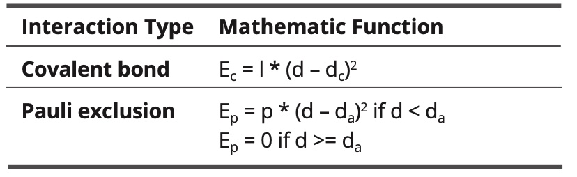
Table 6. Intramolecular interactions.
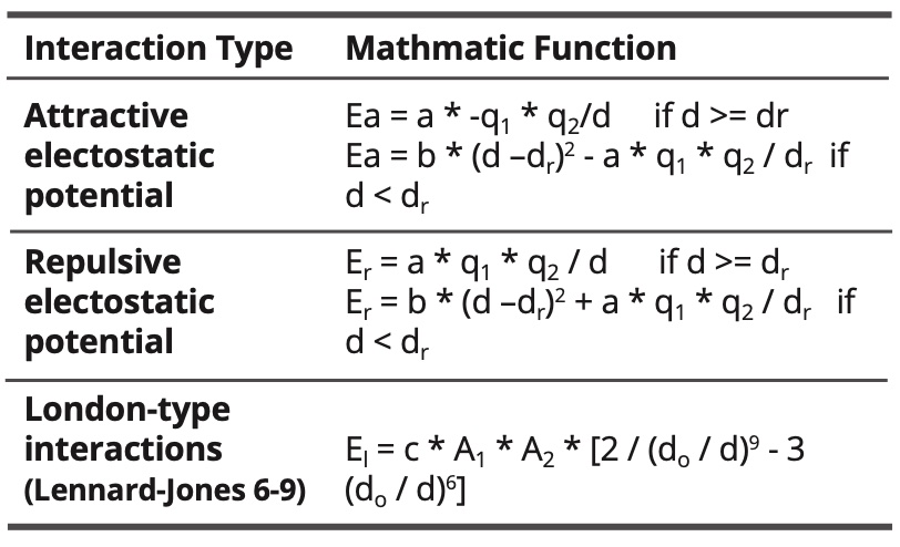
Table 7. Intramolecular interactions.
Where:
d is the distance between atoms
dc is the covalent distance
dc = rc1 + rc2 whit rc1 and rc2 the covalent radii of the atoms
da = ra1 + ra2 with ra1 and ra2 the atomic radii of the atoms
dr is a reference distance in electrostatic interactions
do is the van der Waals distance
do = ro1 + ro2 with ro1 and ro2 the van der Waals radii of the atoms
A1 and A2 are the polarizabilities of the atoms
The constants l, p, a, b and c are fitted.
For the model of the fundamental state of water, the constants are as follows:
Table 8. Constant values for the fundamental water model in nm.
The hydrogen bond has then got the following length:
(11) do—H = rc O + rc d + dr = 0.065 + 0.015 + 0.100 = 0.180 nm
For the models of the excited state of water, the constants are as follows:
Table 9. Constant values for the excited water models in nm.
In the case of the intermediate model, the hydrogen bond has the following length:
(12) do—H = rc O + rc d + dr = 0.065 + 0.085 + 0.100 =
0.250 nm
The step of calculation is 0,005 nm length. It corresponds to 1 pixel in a graphic representation.
Thus:
• The van der Waals radius of the oxygen atom is equal to 0.140 / 0.005 = 28 pixels
• The van der Waals radius of the hydrogen atom is equal to 0.120 / 0.005 = 24 pixels
• The chemical bond length O-H is equal to 0.100 / 0.005 = 20 pixels
When the unit of length is expressed in calculation steps, the adjustable constants of the mathematical formulas have the following values:
Table 10. Values of adjustable constants.
The parametrized polarizabilities and charges of the atoms and electronic free doublets are as follows:
Table 11. Simulated values of charges and polarities.
In the forced model, the electrostatic dipolar intermolecular interactions are completely annihilated (but not the electrostatic dipolar interactions with the electric field). Thus, the polarizability of the oxygen atom is increased to compensate partially the resulting decrease in intermolecular interactions.
Relationship between simulated energy and the real energy:
In the simulation program, according to the simulated length units chosen and the adjustable constant values, the relationship between the simulated energy values and those expressed in J / mol is as follows:
(13) Esimulated = 26.7 E (J /mol)
Note: In the case of the total energy of a nano-droplet, the mole of entities considered in the conversion is a mole of nano-droplets.
The relationship between the simulated temperature and the temperature expressed in kelvins is as follows:
(14) Tsimulated = 0.00741 T(K)
In the simulations the perfect gas constant is equal to 30000.
We have the following relation:
(15) E(J/mol) / [R(J/mol.K) * T(K)] = Esimulated /
[30000 * Tsimulated]
Note: At 20°C or 293 K, Tsimulated = 2.17
Table 12 gives the dimensions of the cubic simulation boxes for the different sizes of nano-droplets, given that the ground-state water density is 1,200 and the density of the water in the state excited is equal to 0.800.
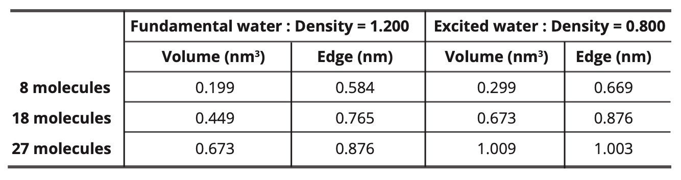
Table 12. Dimensions of the cubic simulation boxes.
Acknowledgements
I acknowledge Professor Marc Henry of the University of Strasbourg and president of the association Natur’Eau Quant for his help to perform this work and his proposition for its publication.
References
1) R Arani, I Bono, E Del Guidice, G Preparata, “QED Coherence and the Thermodynamic of Water” MITH 93 / 3
2) C A Yinnon, T Yinnon, “Domains in aqueous solutions: Theory and Experimental Evidence”, Modern Physics Letters B 23(16) June 2009
3) E Tiezzi, M Catalussi, N Marchettini, “The Supramolecular Structure of Water: NMR studies”, International Journal of Design & Nature and Ecodynamics 5(1):10-20 · May 2010.
4) A Deb, G F Reiter, “Quantum coherence and temperature dependence of the anomalous state of nanoconfined water in carbon nanotubes.” Chemical Science.
5) P Madl, P Kolarž, E Del Giudice, A Tedeschi, A Hartl, M Gaisberger, W Hofmann, “The formation of coherence domains for aerosolized water molecules at alpine waterfalls – Part-1.”
6) E Del Guidice, G Preparata, “Coherent Dynamics in Water as a Possible Explanation of Biological Membranes Formation.” Journal of Biological Physics 20; 105-116, 1994
7) C Messori, “The Super-Coherent State of Biological Water”, Open Access Library Journal 2019, Volume 6, e5236, ISSN Online 2333-9721, ISSN Print 2333-9705
8) C W SMITH, “Quanta and Coherence Effects in Water and Living Systems.” The Journal of Alternative and Complementary Medicine Volume 10 Number 1, 2004, pp 69-78.
9) L Montagnier, J Aissa, E Del Guidice, C Lavallee, A Tedeschi, G Vitiello, “DNA Waves and Water,” Journal of Physics : Conference Series, 306, 012007 arXiv : 1012.5166v1
10) I Bono, E Del Guidice, L Gamberale, M Henry, “Emergence of Coherent Structure in Liquid Water.” Water 2012, 4, 510-532
11) L S Martseniuk “The Effect of Interactions of Coherent Water Systems with Low Intensive Electromagnetic Radiation”, 12th international conference “Interaction of radiation with solids”, September 19-22, 2017, Minsk, Belarus
12) P Renati, Z Kovacs, A De Ninno, R Tzenkova, “Temperature dependence analysis of NIR spectra of liquid water confirms the existence of two phases, one of which is in coherent state,” Journal of Molecular Liquids, Volume 292, October 2019, 111449
13) D C Rapaport, “The Art of Molecular dynamic Simulation,” Cambridge University Press 2004, 594 pages
14) Cao Q, “Contact dynamics of nanodroplets in carbon nanotubes: effects of electric field, tube radius, and salt ions.” Microfluid Nanofluid 22, 98 (2018)
15) Coudert F X, Cailliez F, Vuillemier R, Fuchs A H, Boutin A, “Water nanodroplets confined in zeolithe pores,” Journal of Faraday Discussions, 141, 2009
16 Mingya Zhang, Lijun Ma, QingWang, Peng Hao, XuZheng, “Wettability behavior of nanodroplets on copper surfaces with hierarchical nanostructures,” Colloids and Surfaces A: Physicochemical and Engineering Aspects, Volume 604, 5 November 2020, 125291
17) W H Keesom, “The Second Virial Coefficient for Rigid Spherical Molecules whose Mutual Attraction is Equivalent to that of a Quadruplet Placed at its Center”, Proceedings of the Royal Netherlands Academy of Arts and Sciences 1915, 18, 636-646
18) F London, “The General Theory of Molecular Forces”, Transaction of the Faraday Society, 1937, 33, 8-26
19) Kaatze U, Behrents R, Pottel R, “Hydrogen network fluctuations and dielectric spectrometry of liquids.” Journal of Non-Crystalline solids, volume 305, issue 1, p19-28, July 2002,
20) Handbook of Chemistry and Physics, 54th edition 1973-1974
21) M W Mahoney, W L Jorgensen, “A Five Site Model for Liquid Water and the reproduction of the Density Anomaly by Rigid Nonpolarizable Potential Functions,” Journal of Chemical Physics, 2000, 112, i 20, 8910-8922
22) J E Jones, S Chapman, “On the Determination of Molecular Fields – II, From the Equation of State of a gas,” Proceedings of the royal society A, Mathematical Physical and Engineering Science 1924, 106, i 738
23) Cole, KS; Cole, RH (1941). « Dispersion et absorption dans Diélectriques – I Alternant caractéristiques actuelles ». J. Chem. Phys. 9 : 341-352.
24) Cole, KS; Cole, RH (1942). « Dispersion et absorption dans Diélectriques – II Caractéristiques courant continu ». Journal of Chemical Physics. 10: 98-105.
25) R M Hill, L A Dissado, “Debye and non-Debye Relaxation”, J Physics C : Solid State Phys. 1985, 18, 3829-3836.
26) Ji-Xin Cheng*†, Sophie Pautot‡§, David A. Weitz‡, and X. Sunney Xie “Ordering of water molecules between phospholipid bilayers visualized by coherent anti-Stoke Raman scattering microscopy,” Proceedings of National Academy of Sciences, Edited by Robin M. Hochstrasser, University of Pennsylvania, Philadelphia, PA, and approved June 23, 2003 (received for review April 15, 2003), 100/17/9826
27) F L Leite, C C Bueno, A L Da Roz, E C Ziemath, O N Oliveira Jr, “ Theoretical Models for Surface and Adhesion and their measurement Using Atomic Force Microscopy,” International Journal of Molecular Science 2012, 13(10), 12773-12856
28) P H Blustin, “A Floating Gaussian Orbital Calculation on argon hydrochloride (Ar HCl)”, Theoretica Chimica Acta, 1978, 47 (3), 249-257
29) Naserifar S, Goddart III W.A, “Liquid water is a dynamic polydisperse branched polymer” Proceedings of the National Academy of Sciences of the United States of America Journal Volume: 116 Journal Issue: 6; Journal ID: ISSN 0027-8424