
 Determinants of Faraday Wave-Patterns in Water Samples Oscillated Vertically at a Range of Frequencies from 50-200 Hz
Merlin Sheldrake* & Rupert Sheldrake
Keywords: Faraday wave, pattern formation, vibrational mode, catastrophe theory, bifurcation, analogue model, morphogenesis, parametric oscillation, nonlinear dynamic system
Received: July 13, 2017; Revised: September 6, 2017; Accepted: September 15, 2017; Published: October 25, 2017; Available Online: October 25, 2017
Abstract
The standing wave patterns formed on the surface of a vertically oscillated fluid enclosed by a container have long been a subject of fascination, and are known as Faraday waves. In circular containers, stable, radially symmetrical Faraday wave-patterns are resonant phenomena, and occur at the vibrational modes where whole numbers of waves fit exactly onto the surface of the fluid sample. These phenomena make excellent systems for the study of pattern formation and complex nonlinear dynamics. We provide a systematic exploration of variables that affect Faraday wave pattern formation on water in vertical-walled circular containers including amplitude, frequency, volume (or depth), temperature, and atmospheric pressure. In addition, we developed a novel method for the quantification of the time taken for patterns to reach full expression following the onset of excitation. The excitation frequency and diameter of the container were the variables that most strongly affected pattern morphology. Amplitude affected the degree to which Faraday wave patterns were expressed but did not affect pattern morphology. Volume (depth) and temperature did not affect overall pattern morphology but in some cases altered the time taken for patterns to form. We discuss our findings in light of René Thom’s catastrophe theory, and the framework of attractors and basins of attraction. We suggest that Faraday wave phenomena represent a convenient and tractable analogue model system for the study of morphogenesis and vibrational modal phenomena in dynamical systems in general, examples of which abound in physical and biological systems.
Introduction
When fluid enclosed by a container is subjected to a vertical oscillation, standing waves arise. These standing waves, which depend on reflections from the edge of the container, are known as Faraday waves (Miles and Henderson, 1990). At some frequencies and amplitudes they form highly ordered patterns, while at others they give rise to chaotic dynamics (Simonelli and Gollub, 1989). Faraday wave phenomena make excellent systems for the study of pattern formation because of the high degree of control compared with other pattern-forming systems such as convection or chemical reactions (Huepe et al., 2006), and the great richness and variety of patterns that are possible (Topaz et al., 2004; Rajchenbach and Clamond, 2015). Thus, complex nonlinear phenomena can be explored using a relatively simple experimental device.
Faraday waves and similar resonant phenomena have been the subject of fascination for several centuries. The patterns formed by sound vibrations were described by Leonardo da Vinci, who found that dust particles formed mounds and hillocks when the underlying surface was vibrated (Winternitz, 1982). Similar phenomena were experimentally and observationally researched by Galileo Galilei (1668), Robert Hooke (Inwood, 2003), Ernst Chladni (Chladni, 1787; Waller and Chladni, 1961), Michael Faraday (Faraday, 1831), and Lord Rayleigh (Rayleigh, 1883; 1887).
Faraday and Rayleigh found that the transverse waves excited on the surface of a vertically vibrated fluid oscillated at half the excitation frequency (Faraday, 1831; Rayleigh, 1883). The 2:1 ratio between driving frequency and oscillatory response is characteristic of parametric resonance (Douady and Fauve, 1988; Bechhoefer et al., 1995). A familiar analogy is a child’s swing. If the swing is given a push when it reaches its highest point on one side, and then another push when it reaches the other extreme, these two pushes will help it complete one back-and-forth cycle, and the swing will oscillate at half the excitation frequency.
Standing waves on the surface of fluids are formed when the driving amplitude exceeds a critical threshold (Bechhoefer et al., 1995). Above this point—the so-called Faraday instability—there is a bifurcation from a single state of motion of the free surface of the liquid to multiple states of motion, such that the surface of the liquid might be rising or falling (Miles and Henderson, 1990). Faraday wave patterns are influenced both by properties of the liquid sample, such as the diameter and shape of the container, and the viscosity of the fluid (intrinsic factors), and properties of the oscillation such as excitation frequency and amplitude (extrinsic factors; Abraham, 1976).
Oscillating fluid samples in enclosed containers have particular modes of vibration, in which whole numbers of waves fit exactly onto the surface (Ball, 2009). These Faraday wave modes arise from a combination of the outgoing waves excited by the driving frequency and the waves reflected from the vertical wall of the cell, and depend on the frequency and amplitude of the excitation and the diameter of the cell. They are resonant patterns in the same sense that standing waves in wind instruments such as flutes are resonant patterns of vibration. Faraday waves in fluids are also analogous to the patterns formed by vibrating solid particles on metal plates described by Ernst Chladni in 1787 (Chladni, 1787; Waller and Chladni, 1961). In Chladni’s figures, the patterns are revealed by particles accumulating along the nodal lines, which are parts of the plate that are neither moving upwards nor downwards, and form “a spiderweb of motionless curves” (Abraham, 1976). By contrast, in samples of liquid subjected to vertical vibrations, patterns appear as oscillations of standing waves, with any given point flipping between peak and trough.
Much of the research on Faraday waves has focused on attempts to characterize them mathematically, using theoretical approaches based on equations stemming from physical theories, well-reviewed in Ibrahim (2015). However, the predictions made by such mathematical models often disagree with experimental results, or else make predictions that are only accurate under restricted conditions (Miles and Henderson, 1990; Bechhoefer et al., 1995). For example, an approach based on the Mathieu equations, which are used to model parametric resonance, was only partially successful in modelling surface waves because it could not take into account fluid viscosity (Benjamin and Ursell, 1954; Bechhoefer et al., 1995). Other investigations have used the Navier-Stokes equations (which describe the flow of viscous substances) to characterize Faraday wave pattern dynamics (eg. Kumar and Tuckerman, 1994). But solving Navier-Stokes equations for such complex dynamical systems presents an enormous computational challenge. Furthermore, even if the equations can be solved, these models cannot account for perturbations or disruptions that the system is likely to encounter in the real world (Ball, 2009).
These problems with classical mathematical approaches have led some to adopt a more phenomenological approach towards Faraday wave systems, looking at the empirical patterns themselves, as opposed to the theoretical modes of these patterns. For the most part, these studies explore vibrational modes and the transitions between them using analogue stimulation and direct observation. For example, Abraham (1975) conceived of the experimental Faraday wave system as more than a way to verify the predictions of equation-based models. Rather, he understood it as a top-down exploratory process, and described his experimental system as “an analogue computer simulating the Navier-Stokes equations” (Abraham, 1975). Another way to understand this approach is in the context of Richard Feynman’s call for a “method of understanding the qualitative content of equations,” observing that “today we cannot see that the water flow equations contain such things as the barber pole structure of turbulence that one sees between rotating cylinders” (Feynman et al. 1964). Following this empirical approach, some researchers have focused on the Faraday wave patterns that interact with each other on the boundaries between different modes (Ciliberto and Gollub, 1984; Simonelli and Gollub, 1989). Some have used the Faraday wave system to model the onset of chaotic behavior at these boundaries, or at high amplitudes (Tufillaro et al., 1989; Gluckman et al., 1993). Others have used comparable systems to model biological phenomena, most notably the transduction of sound in the cochlea, which underlies our own sense of hearing (von Bekesy, 1960). Experimental work in this area was influenced by Hans Jenny (2001), who investigated the effects of vibrations on the patterns produced by vibrating fluids, pastes and powders.
Faraday wave systems provide an excellent arena for the physical modelling of prevalent theoretical frameworks in the physical and biological sciences. These include: i) the widespread mathematical procedure, the Eigendecomposition of the Laplace operator, which lies at the heart of theories of heat, light, sound, electricity, magnetism, gravitation and fluid mechanics (Stewart, 1999); ii) the well-known reaction-diffusion model of Turing (1952), which is based on standing or oscillatory chemical waves (ie. peaks and troughs), and underpins much contemporary understanding of biological morphogenesis (Ball, 2015); and iii) the catastrophe theory of René Thom, which provides a mathematical underpinning for the modelling of sudden transitions, or catastrophes, between alternative states (Thom, 1975), and which has been experimentally applied to Faraday wave systems by Abraham (1972). Examples of systems that exhibit complex nonlinear dynamics and modal behavior analogous to those in the Faraday wave system are widespread and range from the laser-induced vibrations of ions in a crystal lattice (Britton et al., 2012) to cortical activity in the human brain (Atasoy et al., 2016).
Despite the practical and theoretical value of the experimental Faraday wave system to numerous areas of the physical and life sciences, to our knowledge there are no investigations into the factors that influence the formation of Faraday wave patterns across a wide frequency range. Some studies have examined the effects of square, rectangular and pentagonal as opposed to circular fluid reservoirs (Douady and Fauve, 1988; Simonelli and Gollub, 1989; Torres et al., 1995), and some refer to the effect of fluid volume (Henderson and Miles, 1991), temperature (Bechhoefer et al., 1995), topography of the reservoir bottom (Kalinichenko et al., 2015), and liquid purity (Henderson et al., 1991; Henderson, 1998). However, these studies do not systematically report the effects of the major factors determining overall pattern morphology.
Here we present a systematic exploration of variables that affect Faraday wave pattern formation on water in vertical-walled circular containers. We investigated the effects of amplitude, frequency, volume (or depth), temperature, and atmospheric pressure on the morphology of Faraday wave patterns. We also developed a novel method for the quantification of the time taken for patterns to reach full expression following the onset of excitation. We studied the spectrum of vibratory modes across a wide frequency range, from 50-200 Hz. In addition, we determined the stability boundaries around three sample frequencies.
Methods
Experimental Apparatus
We generated Faraday waves by vertically oscillating a liquid sample held in a cylindrical container, or visualizing cell, using sound frequencies. We used the Cyma-Scope instrument (Sonic Age, Cumbria, UK). The cell was vertically oscillated using a voice coil motor (VCM) optimized to operate between 50-200 Hz. Inherent resonances in the electromechanical system of the VCM were damped internally by enclosing the back pressure of the VCM in an infinite baffle arrangement and by inserting a thermal compressor into the VCM’s circuit. Resonances were further controlled using a Klark Technik Square One thirty-band graphic equalizer (Klark Technik, Kidderminster, Worcestershire, UK). A diagram of the signal path is provided in Figure 1.

Figure 1. Diagram of the signal path and experimental apparatus.
The VCM was driven with frequencies defined by a function generator (Aim TTi, Huntingdon, Cambridgeshire, UK). Unless otherwise stated, we used sinusoidal oscillations, although we also evaluated the effect of using square and triangle wave forms generated by the function generator on pattern formation. The amplitudes of the wave forms were defined in terms of voltage from the function generator. The function generator did not provide sufficient power on its own and so the signal was amplified using a Lindell Audio AMPX Class A amplifier (Lindell Audio, Phuket, Thailand). To achieve precise and programmable control of the amplitude, we included a Volcano attenuator (Sound Sculpture, Bend, OR, USA) which used a resistor selector circuit controlled by MIDI control change messages to attenuate the signal to the required amplitude. We used as a proxy for amplitude the magnitude of the signal delivered to the VCM in millivolts (mV), measured using a voltmeter (Hioki, Nagano, Japan) connected across the output terminals of the amplifier. Higher excitation frequencies required greater amplitudes to excite the sample to the point of Faraday instability and pattern formation. We found the appropriate amplitude by trial and error.
We used cells of three different diameters. The diameters were 10.00 mm, 24.25 mm, and 49.50 mm. Unless otherwise stated, all results presented are obtained using the medium cell (diameter = 24.25 mm). Cells were made of fused quartz glass, with sand-blasted matt black surface on the bottom so that the light used for visualizing was reflected from the surface of the liquid only. Cells were cleaned using 100% ethanol, and rinsed with deionized water (resistivity 18 M-ohms). We used the same kind of deionized water for our liquid samples when performing experimental oscillations. The cell was illuminated from above by a ring of LEDs. Wave patterns were imaged from above using a Canon EOS SLR 7D Mark II with a Canon 100 mm f2.8 macro lens (Canon, Tokyo, Japan), shooting at 25 frames per second (fps). The camera was levelled to ensure that the line of sight was perpendicular to the surface of the liquid, thus avoiding parallax errors. The high-speed video recordings used to ascertain the dominant frequency of the excited surface ripples were recorded using a Canon FS7 (Canon, Tokyo, Japan) with the same lens as above, shooting at 150 fps.
Data Processing and Analysis
Classification of pattern morphology: We classified the morphology of the patterns resulting from the Faraday wave forms based on fold symmetry. For example, a regular six-pointed pattern would be classified as having six-fold symmetry. This is a straightforward and inclusive taxonomic criterion that accounts for similarities and differences in the overall morphology of patterns.
Evaluation of time to full expression of pattern (TFE): We define the TFE as the time taken for the pattern to reach full expression following the onset of the excitation frequency. We devised a semi-automated, objective procedure for defining the point at which patterns had reached full expression. Briefly, videos were cropped, so that only the circular surface of the water sample was visible. Video frames were then thresholded so that every pixel was either black or white, and the mean gray value of each frame calculated (mean value = black pixels + white pixels / total number of pixels). Because the patterns showed up as light on a dark background (eg. Figure 3), frames with fuller expression of the pattern had higher gray values than those where the pattern was less expressed. The standard deviation of the mean gray values was plotted against video frame to produce a profile plot of the video (Figure 2). We used the standard deviation of the mean gray value rather than the mean gray value itself because the resulting profile plots were less noisy. Profile plots clearly indicated the point at which a stable pattern had formed, and were used to define a 95% confidence area around the gray values of the pattern in full expression. The time at full expression was defined as the time at which the gray value of a given frame reached the lower 95% confidence limit of the gray values of the pattern in full expression (ie. the time at which there was a statistically significant probability—at α = 0.05—that a frame’s gray value had reached the level of those where the pattern was fully expressed). TFE was then calculated by subtracting the time at onset of excitation from the time at full expression. Image processing was conducted in R v. 3.1.2 (R Development Core Team, 2014), using the package EBImage (Pau et al., 2010). Custom functions were written to execute the procedures outlined above.

Figure 2. Method used to evaluate time taken for the pattern to reach full expression following the onset of the excitation frequency (time to full expression, or TFE). In a, video frames are displayed, showing the onset of the excitation frequency (i), and the onset of full expression of the pattern (ii). b is a profile plot showing the standard deviation of the mean gray value of each video frame as a function of frame number. The onset of the excitation frequency (i), and the onset of full expression of the pattern (ii) are marked. Red horizontal lines show the mean (solid line) and 95% confidence area (dashed lines) around the standard deviation of the mean gray values of the pattern in full expression.
Effect of Amplitude on Pattern Formation
To ascertain the effect of amplitude on pattern formation we oscillated a 2.5 ml sample of water at incrementally increasing amplitudes at each of three sample frequencies, 56, 111 and 180 Hz, replicated three times. The sample of water was changed between each trial. We calculated the TFE using the method described above. We evaluated the effect of amplitude on the variability of the TFE by modelling the standard deviation of the TFE of the three replicates at each amplitude as a function of amplitude. We used linear models and ran separate models for each of the three frequencies. All models met assumptions of normality and homogeneity of variances.
Effect of Sample Volume (Depth) on Pattern Formation
To explore the effect of volume on pattern formation, we oscillated four volumes of water (1.5 ml, 2.5 ml, 3.5 ml and 4.5 ml) at each of the three sample frequencies, replicated three times. The sample of water was changed between each trial. We calculated the TFE using the method described above, and evaluated the effect of sample volume on TFE using linear models (n = 12), running separate models for each of the three frequencies. All models met assumptions of normality and homogeneity of variances. All statistical analysis was conducted in R v. 3.1.2 (R Development Core Team, 2014).
To measure evaporative loss of water we oscillated water for 1 minute, 5 minute and 10 minute periods, and measured the mass of the sample before and after oscillation. The 10 minute period substantially exceeded the length of time that any sample was oscillated in the course of these investigations.
Effect of Temperature on Pattern Formation
To investigate the effect of temperature on pattern formation, we oscillated samples of water at each of the three sample frequencies at five temperatures (5oC, 10oC, 15oC, 20oC, 25oC, and 30oC), replicated three times. The sample of water was changed between each trial. Temperature was controlled using a thermostatically controlled incubator (LMS, Sevenoaks, Kent, UK). We measured the temperature of parallel samples of water before oscillation to ensure that the samples had fully equilibrated. Parallel samples were used to take temperature readings to avoid changing the temperature of the actual sample by the insertion of the thermometer. We calculated the TFE using the method described above, and evaluated the effect of sample temperature on TFE using linear regression, running separate models for each of the three frequencies (n = 18). All models met assumptions of normality and homogeneity of variances.
Effect of Frequency on Pattern Formation
To ascertain the effect of frequency on pattern formation we oscillated water samples of 2.5 mls from 50-200 Hz, increasing in 1 Hz increments, changing the sample of water every 10 trials, i.e. every 10 Hz (preliminary experiments demonstrated that pattern morphology was unaffected by prior oscillation).
Determination of Stability Boundaries
In a Faraday wave system, liquid oscillates in a single stable pattern at certain frequencies when the amplitude is above a critical threshold (Ibrahim, 2015). These critical amplitudes vary as a function of excitation frequency. Plots of critical amplitudes as a function of excitation frequency are known as stability curves, and represent the stability boundary of the system (Simonelli and Gollub, 1988; 1989; Douady, 1990; Henderson and Miles, 1991). To describe the stability boundaries of our system we oscillated water samples at particular frequencies at amplitudes well above those required for pattern formation. We then slowly reduced the amplitude with a slider until the pattern disappeared. We defined this value as the critical amplitude required to sustain a given Faraday wave pattern. We repeated this at 0.5 Hz intervals both below and above each of our three sample frequencies. We plotted the critical amplitude values as a function of excitation frequency to describe stability curves around each of our three sample frequencies. This approach is similar to that described in Simonelli and Gollub (1988).
We asked whether reducing the amplitude could shift the pattern to an alternative form when close to the transition point between stability curves. To test this we used two frequencies (115 Hz and 184 Hz) close to the boundary between two stability curves. At these frequencies, one of two alternative patterns formed unpredictably. We conducted four trials per sample of water, on six samples of water per frequency (a total of 48 trials), recording which pattern formed. After the pattern was fully expressed, we slowly reduced the amplitude, recording any change in the pattern that occurred.
Effect of Atmospheric Pressure on Pattern Formation
To investigate the effect of atmospheric pressure on pattern formation, we excited samples of water at the two transition frequencies (115 Hz and 184 Hz). We conducted four trials per sample of water, on six samples of water per frequency (a total of 48 trials), recording which pattern formed. This was performed on five days with differing atmospheric pressures (ranging from 987-1021 mm). Between each sample, the vessel was cleaned with ethanol, rinsed with deionized water, and dried.
Data were analyzed as the proportion of trials for a given sample forming one or the other of the patterns using generalized linear models (GLMs) with atmospheric pressure and temperature as predictors (the temperature varied only slightly across the trial days, from 19.1-21.6 oC). The data were overdispersed (the residual deviance was greater than the number of degrees of freedom), and so quasibinomial error structures were used (Crawley, 2007). Significance was assessed using χ2 tests.
Results
Morphology of the Three Sample Frequencies
In initial tests we explored a wide range of frequencies, and selected three that gave repeatable patterns in order to investigate those factors affecting pattern formation in more detail. We later returned to a systematic examination of the effects of frequency on pattern over the entire range of our apparatus, from 50-200 Hz, as discussed below.
We chose three frequencies that produced patterns with different morphologies. At 56 Hz, the pattern showed six-fold symmetry; at 111 Hz, the pattern showed ten-fold symmetry; and at 180 Hz the pattern showed fourteen-fold symmetry (Figure 3, composite images). The overall patterns were composites of two alternating phases of oscillation (Figure 3, phases I and II), whereby peaks became troughs, and troughs peaks. We could see these alternating peaks and troughs only by using fast shutter speeds; at the normal shutter speed of 1/30 second, the pictures were a composite of the peak and trough patterns. Thus the six-fold symmetry we observed at 56 Hz represents a standing wave pattern of mode three, with three alternating peaks and troughs, the ten-fold symmetry at 111 Hz mode five, and the fourteen-fold symmetry at 180 Hz mode seven.
We measured the rate of oscillation by examining frame-by-frame photographs from high-speed films, and found that the dominant frequency of the Faraday waves was half the excitation frequency (in other words, the first subharmonic of the excitation frequency: f = fo/2) (Francois et al., 2013). For example, at an excitation frequency of 56 Hz, the frequency of oscillation of the water sample was 28 Hz. This confirmed the results in the classic papers by Faraday (1831) and Rayleigh (1883).

Figure 3. The three sample frequencies resulted in different pattern morphologies shown as composite images (left-hand panels), and images of alternating phases (center and right-hand panels). 56 Hz resulted in six-fold symmetry, 111 Hz in ten-fold symmetry, and 180 Hz in fourteen-fold symmetry.
 Figure 4. Amplitude altered the degree to which patterns were expressed, and in all but two cases did not affect the overall morphology of the pattern. Patterns formed over a range of twelve amplitudes are shown for each of the three sample frequencies. Amplitude is reported beneath each panel in millivolts (mV). Instances in which multiple patterns formed at a given amplitude are marked with horizontal bars and emboldened millivoltages.
Effects of Amplitude
We observed a minimum amplitude below which no pattern formed, and a maximum amplitude above which patterns became overdriven and severely distorted. Within the range of amplitudes that resulted in stable pattern formation, variation of the excitation amplitude did not alter the overall morphology of the pattern. For example, the six-fold 56 Hz pattern remained six-fold across an amplitude range of 65 mV to 491 mV. Nonetheless, amplitude did alter the degree to which patterns were expressed (Figure 3). At 111 Hz and 180 Hz, at the highest amplitude resulting in a coherent pattern, the pattern became unstable and shifted to an alternative pattern. In the case of 111 Hz, the 10-fold pattern shifted to a 16-fold pattern. In the case of 180 Hz, the 14-fold pattern shifted to an unstable 20-fold pattern (Figure 3c).
Amplitude altered the time taken for the pattern to reach full expression following the onset of excitation (time to full expression, or TFE), with higher amplitudes causing the pattern to form more quickly until a minimum TFE was reached (Figure 5). Variation between replicate trials was greater at lower amplitudes at all three frequencies (linear regression: 56 Hz; T1,17 = -2.76; P = 0.01; 111 Hz; T1,14 = -3.41; P = 0.004; 180 Hz; T1,11 = -2.87, P = 0.02; Figure 5).

Figure 5. The time taken for patterns to reach full expression after the start of excitation (TFE) decreased with increasing amplitude (a), as did the variation in TFE between replicates (b-d). In a, separate curves are plotted for each of the three sample frequencies, with error bars depicting the standard deviation of the TFE for three replicates at each amplitude. b-d show significant negative relationship between the standard deviation of the TFE and amplitude. In b-d, lines are the fitted response of separate linear models for each of the three frequencies, with gray bands depicting 95% confidence intervals. 56 Hz (gray); T1,17 = -2.76; P = 0.01; 111 Hz (maroon); T1,14 = -3.41; P = 0.004; 180 Hz (blue); T1,11 = -2.87, P = 0.02.
Effects of Wave Form
The wave form (sine wave, square wave or triangle wave) of the driving frequency did not alter the overall morphology of the pattern. For example, the six-fold 56 Hz pattern remained six-fold when oscillated using sine, square or triangle waves (Figure 6).

Figure 6. The wave form (sine wave, square wave or triangle wave) of the driving frequency did not alter the overall morphology of the pattern at any of the three sample frequencies.
Effects of Sample Volume and Depth
The sample volume, and thus depth, of oscillating water did not alter the overall morphology of the pattern. For example, the six-fold 56 Hz pattern remained six-fold across a volume range of 1.5 mls to 4.5 mls with only marginal changes in the degree to which the pattern was expressed (Figure 7). Higher volumes of water increased the time taken for the pattern to reach full expression (linear regression: 56 Hz; T1,10 = 2.14; P = 0.06; 111 Hz; T1,10 = 5.81; P < 0.001; 180 Hz; T1,10 = 5.89, P < 0.001; Figure 8).

Figure 7. The volume, and thus depth, of oscillating water had a marginal effect on the degree to which patterns were expressed, and did not affect the overall morphology of the pattern. Patterns formed at four volumes (1.5, 2.5, 3.5 and 4.5 ml) are shown for each of the three sample frequencies.

Figure 8. The time taken for the pattern to reach full expression after the start of forced oscillations (TFE) increased with higher volumes, and thus depths, of water. Lines are the fitted response of separate linear models for each of the three frequencies, with gray bands depicting 95% confidence intervals, solid lines indicating a significant relationship (P < 0.05), and dotted lines indicating a marginally significant relationship (0.5 < P < 0.1). 56 Hz (gray); T1,10 = 2.14; P = 0.06; 111 Hz (maroon); T1,10 = 5.81; P < 0.001; 180 Hz (blue); T1,10 = 5.89, P < 0.001.
Evaporative loss of water during experimental time periods was minimal: over a ten minute period (longer than any single water sample was used for in this investigation) a mean of 0.003 g of water (n = 6; std. dev. = 0.005) was lost from the quartz cell at standard operating temperature and pressure. This represents 0.13% of the total mass of water in the cell.
Although at lower volumes the time taken for the pattern to reach full expression was less (Figure 8), volume had minimal effects on pattern morphology (Figure 7). This indicates that any evaporative loss of water over the course of our experiments – less than 0.13% – is unlikely to affect the pattern formed, since far larger changes – between -40% and +180% of the standard volume we used in our experiments – had almost no effect on pattern morphology (Figure 7).
Effects of Temperature
The temperature of the oscillating water and cell did not alter the overall morphology of the pattern. For example, the six-fold 56 Hz pattern remained six-fold across a temperature range of 5-30oC with no noticeable differences in the degree to which the pattern was expressed (Figure 9).

Figure 9. Temperature did not alter the overall morphology of the pattern and had a negligible effect on the degree to which patterns were expressed. Patterns formed at six temperatures (5oC, 10oC, 15oC, 20oC, 25oC, and 30oC) are shown for each of the three sample frequencies.
Temperature had a variable effect on the time taken for patterns to reach full expression. At 56 Hz, increasing temperatures reduced the time taken for the pattern to reach full expression, although this effect was not strong (linear regression: T1,16 = -2.41; P = 0.03; Figure 10). At 111 Hz there was a non-significant trend for temperature to reduce the time taken for the pattern to reach full expression (T1,16 = -1.81; P = 0.09; Figure 10). At 180 Hz there was no effect of temperature on time to full expression (T1,16 = -0.70, P = 0.50; Figure 10).

Figure 10. Increasing temperatures reduced the time taken for the pattern to reach full expression (TFE) at 56 Hz but not at 111 Hz or 180 Hz. Lines are the fitted response of separate linear models for each of the three frequencies, with gray bands depicting 95% confidence intervals, solid lines indicating a significant relationship (P < 0.05), and dotted lines indicating a marginally significant relationship (0.5 < P < 0.1). 56 Hz (gray); T1,16 = -2.41; P = 0.03; 111 Hz (maroon); T1,16 = -1.81; P = 0.09; 180 Hz (blue); T1,16 = -0.70, P = 0.50.
Effects of Excitation Frequency from 50-200 Hz
Pattern morphology was strongly dependent on the excitation frequency, and varied from two-fold to twenty-fold symmetry (Figure 11). Different pattern morphologies appeared in frequency bandwidths, interspersed with frequency bandwidths that resulted in either no patterns or indistinct patterns. In other words, pattern morphology changed discretely while frequency increased continuously. The spectrum of pattern morphologies was broadly consistent across the three repetitions, but showed some variation in the length, and start or endpoint of any given pattern’s bandwidth (Figure 11). There was a highly ordered relationship between excitation frequency and the resulting patterns’ degree of symmetry (Figure 12).

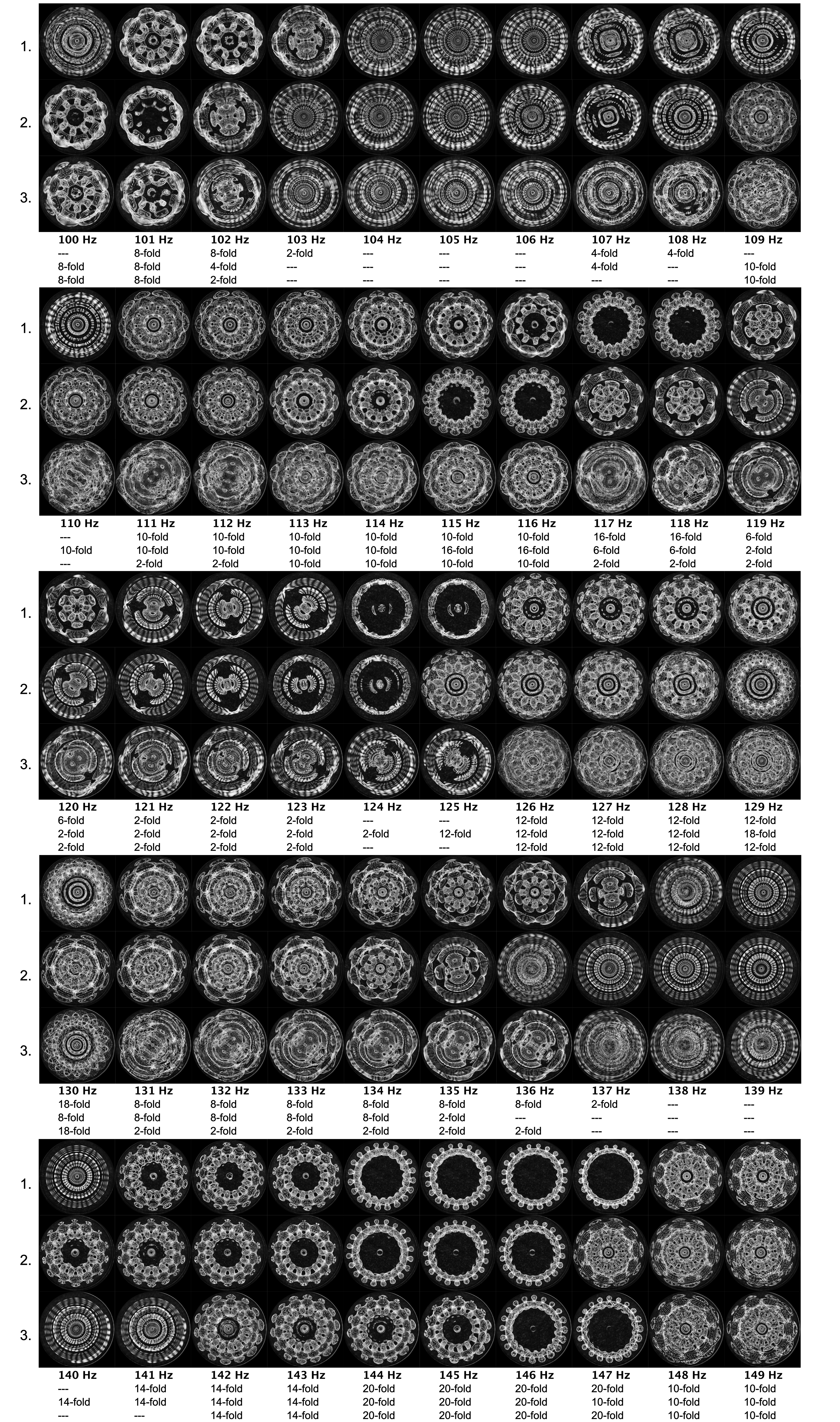

Figure 11. Effect of excitation frequency on pattern morphology using the medium cell (diameter = 24.25 mm) increasing from 50 Hz to 199 Hz in 1 Hz increments (10 Hz per row). The fold symmetry of each pattern (2-fold, 4-fold, etc.) is reported beneath each panel. Rows 1, 2, and 3 are three replicates performed on different days.

Figure 12. Relationship between the excitation frequency and the fold symmetry of pattern formed for the medium cell. The three replicates are represented in light blue through dark blue and show the frequency bandwidths of the patterns. The gray shaded area highlights the patterns of two-fold symmetry which have poorly defined morphology and represent neither developed patterns nor no patterns. Data are the same as those presented in Figure 11.
Determination of Stability Boundaries
The critical amplitude required to sustain a given Faraday wave-pattern varied as a function of excitation frequency. A lower excitation amplitude was required to sustain the pattern at the center of the frequency range at which each pattern was produced than at the edges of this range. The resulting stability curves were thus parabolic, or trough-shaped, with the middle of the frequency range occurring towards the bottom of the trough (Figure 13). Beyond the borders of each trough there were either no patterns or different patterns: the stability curve for 56 Hz did not intersect with an adjacent pattern, while the stability curve for 111 Hz and 180 Hz intersected with adjacent patterns at 113 Hz and 183 Hz respectively (Figure 13). In the regions close to the points of intersection between adjacent troughs, patterns were often unstable. For example at 184 Hz, a 14-fold pattern formed to start with, and then gave way to an unstable 20-fold pattern (Figure 14).

Figure 13. Stability curves around each of the three sample frequencies as described by the relationship between excitation frequency and the critical amplitude required to sustain a given Faraday wave pattern. A lower excitation amplitude was required to sustain the pattern at the center of the frequency range at which each pattern was produced than at the edges of this range. Dotted vertical lines show the three sample frequencies used in this study. Values are the critical amplitude required to elicit a Faraday wave pattern. Filled symbols represent values at which characteristic Faraday wave patterns formed (filled circles = 6-fold pattern; filled triangles = 10-fold pattern; filled squares = 14-fold pattern). Open symbols represent frequencies at which other patterns formed (open triangles = 16-fold pattern; open squares = 20-fold pattern). The patterns themselves are shown beneath the graph and the range of frequencies at which they formed is indicated by gray bars.

Figure 14. Montage of video frames showing the instability between alternative Faraday wave patterns at 184 Hz. The 14-fold pattern was replaced by an unstable 26-fold pattern.
In regions close to the points of intersection between different troughs, patterns sometimes shifted to alternative patterns when the amplitude was slowly reduced. At 115 Hz, the initial pattern (10-fold or 16-fold) transitioned to the alternative pattern in 37.5% of trials (standard deviation = 20%). At 184 Hz, the initial pattern (14-fold or 26-fold) transitioned to an alternative pattern in 25.2% of trials (standard deviation = 20.2%).
Effect of Atmospheric Pressure on Pattern Formation
At 115 Hz, higher atmospheric pressures increased the probability that the higher-order pattern would form (16-fold versus 10-fold: χ2 = 8.0, P = 0.005; Figure 15). At 184 Hz higher atmospheric pressures marginally increased the probability that the higher-order pattern would form (26-fold versus 14-fold: χ2 = 4.7, P = 0.03; Figure 15). There was no effect of temperature on the probability that the alternative pattern would form at either frequency (115 Hz: χ2 = 0.43, P = 0.51; 184 Hz: χ2 = 0.92, P = 0.34).

Figure 15. Atmospheric pressure increased the probability of the higher order pattern forming when samples of water were oscillated at frequencies close to the point of intersection between adjacent stability troughs. At 115 Hz either 10-fold or 14-fold patterns formed. At 184 Hz either 14-fold or 26-fold patterns formed. Values are the probability that the higher order pattern would form, and lines are fitted values of separate generalized linear models for each of the two frequencies, with gray bands depicting 95% confidence intervals. 115 Hz: χ2 = 8.0, P = 0.005; 184 Hz: χ2 = 4.7, P = 0.03).
Effects of Cell Diameter
Cell diameter had a pronounced effect on pattern morphology. Using the small cell (diameter = 10.00 mm) we obtained regular patterns across the 50-200 Hz range, which differed from the patterns obtained using the medium cell (diameter = 24.25 mm). A spectrum of pattern morphologies for the smaller cell is presented in Figure 16. As was the case for the medium cell, there was a highly ordered relationship between excitation frequency and the resulting degree of symmetry of the pattern (Figure 17). Using the large cell we obtained indistinct patterns. At frequencies below ~65 Hz patterns displayed classifiable morphologies, although were somewhat unstable and irregular. At frequencies above ~65 Hz, patterns became more unstable and indistinct, and we were unable to classify them according to fold symmetry. An example is shown in Figure 18.
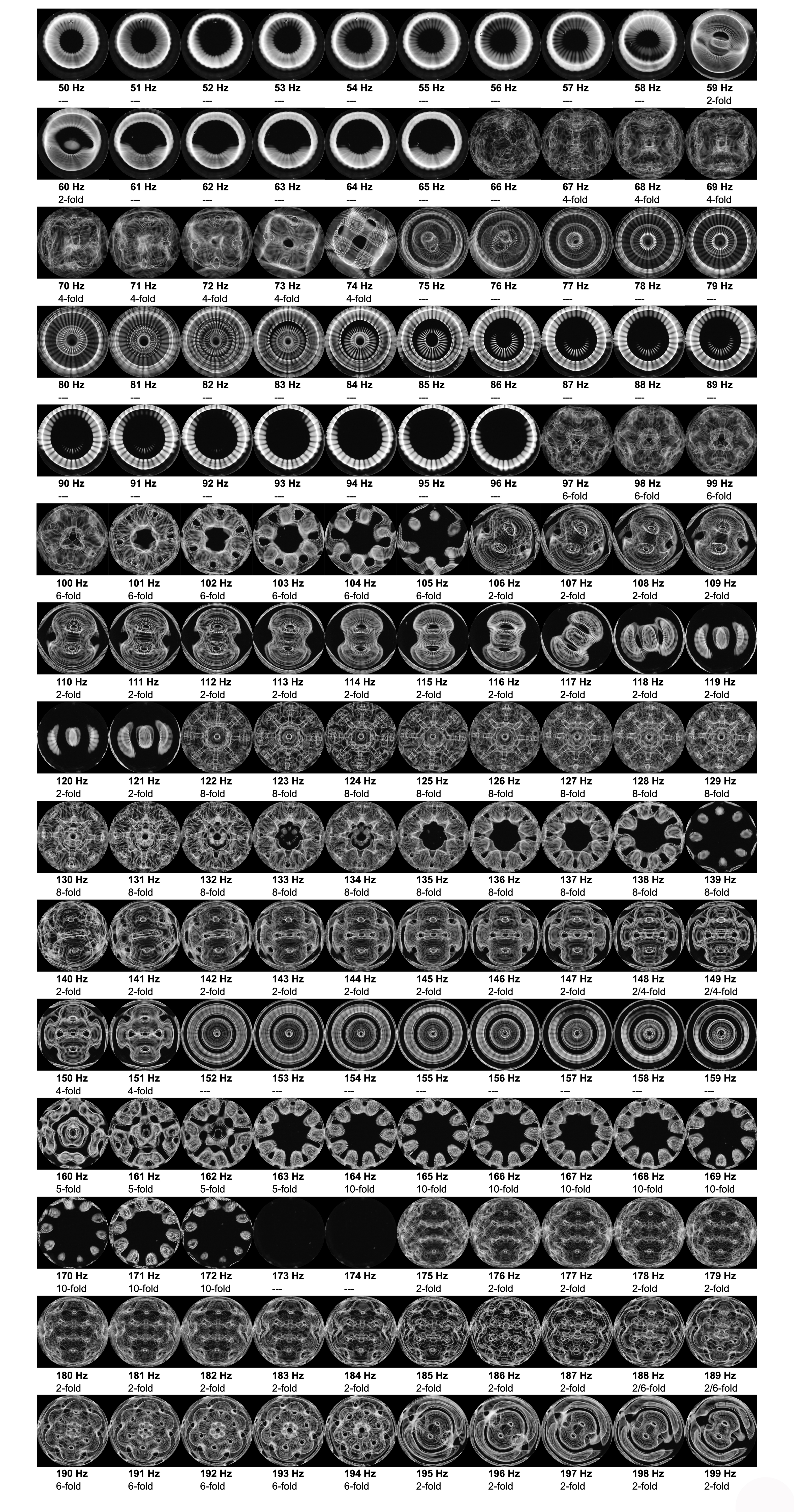
Figure 16. Effect of excitation frequency on pattern morphology using the small cell (diameter = 10.00 mm) increasing from 50 Hz to 199 Hz in 1 Hz increments (10 Hz per row). The fold symmetry of each pattern (2-fold, 4-fold, etc.) is reported beneath each panel.

Figure 17. Relationship between the excitation frequency and the fold symmetry of pattern formed for the small cell. The gray shaded area highlights the patterns of two-fold symmetry which have poorly defined morphology and represent neither developed patterns nor no patterns. Data are the same as those presented in Figure 16.

Figure 18. Patterns formed in the large cell (diameter = 49.50 mm) were irregular and somewhat unstable. At frequencies below ~65 Hz (a and b), pattern morphologies could be classified according to their fold symmetry. At frequencies above ~65 Hz (c and d), pattern morphologies could not be classified.
Discussion
Determinants of Faraday Wave Pattern Morphology
As Abraham (1976) pointed out, Faraday wave pattern morphology depends on i) intrinsic controls, which are properties of the liquid, such as its dimensions, viscosity and elasticity; and ii) extrinsic controls, which are properties of the driving oscillations, such as excitation frequency or amplitude.
We confirm that the morphologies of Faraday wave patterns in water are dependent on both intrinsic and extrinsic controls, most notably: i) the frequency of the forced oscillation (extrinsic), and ii) on the diameter of the fluid reservoir (intrinsic). On the whole, none of the other variables examined, whether intrinsic (fluid volume/depth, and temperature) or extrinsic (amplitude, and wave form) caused changes in pattern morphology, although amplitude altered the degree to which the pattern was expressed (Figure 4), and amplitude, volume, and to a small extent temperature altered the time taken for the pattern to form (Figures 4, 7, 9). The only exceptions occurred when water samples were oscillated at 111 Hz and 180 Hz at very high amplitudes, which caused the Faraday wave patterns to jump to alternative patterns (Figure 4), and at transition frequencies (115 and 184 Hz) when reductions in amplitude brought about transitions between alternative patterns. We discuss this below.
Effect of Frequency on Pattern Morphology
The relationship between excitation frequency and the resulting Faraday wave pattern was discontinuous: when we increased the frequency continuously, the Faraday wave patterns changed discretely, jumping or wobbling between alternative forms, or disappearing altogether at a particular cutoff frequency (Figures 10-11; Abraham, 1976). A familiar analogy is the tuning of a radio. As the tuning frequency is increased continuously, there is a discontinuous series of broadcasts that are tuned into, each a resonant band with a certain bandwidth.
The discontinuous relationship between frequency and Faraday wave pattern demonstrates that the Faraday wave patterns, or attractors—the mathematical description of a Faraday wave pattern (Abraham, 1976)—are discrete and cannot change continuously as the excitation frequency is changed. The bandwidth, or range of frequencies that give rise to a given pattern may thus be thought of as the basin of attraction—the set of initial frequencies that lead asymptotically to the attractor (Simonelli and Gollub, 1988). The basin boundaries, or frequency values at which a small change in the control parameters elicit a significant change in form, may be thought as catastrophic points in the sense of Abraham (1972) and René Thom (1975). Catastrophes may be of different types: Abraham (1972) classes the transition between patterns into “jump” (Hopf-Takens) or “wobble” (Duffing-Zeeman) type catastrophes, both of which we observed (a “jump” from 14-fold to 26-fold is shown in Figure 14, frames 0-93; a “wobble” is shown between alternative forms of a 26-fold pattern in Figure 14, frames 93-165). Thus, the spectrum of patterns formed across the frequency range (Figure 11) are best thought of as describing basins of attraction, separated from each other by catastrophes.
There was a clear systematic relationship between excitation frequency and the fold symmetry of the pattern formed (Figure 12, 17). We observed a similar ascending series in both the medium and the small cell, which suggests that our findings describe a generalisable relationship between excitation frequency and the fold symmetry of Faraday wave patterns for a given diameter of oscillating reservoir. If formalised, this relationship could provide the basis for predicting pattern morphology from excitation frequency and vice versa (for a given liquid medium and reservoir diameter). A similar relationship has been described by Telfer (Web ref. 1). While we offer no formalisation of this relationship here, it seems probable that the repetition of different patterns describes harmonics and subharmonics of the excitation frequency, and their relationship with the diameter of the vessel and intrinsic properties of the liquid medium.
We limit the enquiry presented here to deionized water. Nonetheless, we know from our own investigations and from the literature (Henderson et al., 1991; Henderson, 1998) that pattern morphology is strongly dependent on the properties of the oscillating fluid. For example, at a given excitation frequency and cell diameter, we found patterns of different fold symmetry were formed in water, n-butanol and 1-pentanol (data not shown). Further work is needed to identify whether liquids with different physical properties show systematic relationships similar to the one described here, between excitation frequency and fold symmetry (Figure 12 and 17).
We observed that the amplitude, or energy, required to sustain a given pattern was dependent on frequency: patterns required the lowest amplitude towards the center of their frequency bandwidths, or basins of attraction. At the edges of the frequency bandwidths, greater amplitudes were required to sustain the patterns (Figure 13). Ciliberto and Gollub (1984) described a similar phenomenon, with amplitudes required to sustain a Faraday wave pattern rising at frequencies towards the edge of a pattern’s bandwidth. This relationship may be thought of as a resonance curve, a common way to describe the resonant response of a system (Siebert, 1986).
From another point of view, this relationship between the minimum amplitude required to sustain a given pattern resembles the energy landscape approach used in the study of complex chemical systems such as proteins (Wales, 2003). Both consider the energy of the system (in this case, the minimum amplitude required to sustain a pattern) as a function of form or configuration (in this case the Faraday wave pattern). According to energy landscape approaches, the configuration, or form, of a molecule is funnelled towards a minimum energy state, which can be reached by multiple pathways and intermediate forms (Leopold et al., 1992), analogous to a ball or other such object rolling to the bottom of a valley, and reaching the bottom of the valley no matter which point on the sloped sides of the valley it is released from. Forms, or configurations higher up the energy “funnel” are less stable than those towards the bottom of the funnel. Indeed, we found that the Faraday wave patterns displayed greater stability at the vertex of the parabola than higher up the curve (Figure 14), as did Ciliberto and Gollub (1984).
At the boundaries between adjacent basins of attraction, we observed competition between alternative patterns (Figure 13). A similar phenomenon was reported by Ciliberto and Gollub (1984), who describe competition between alternate patterns in regions close to the point at which neighboring stability curves intersect, giving rise either to slow oscillations between alternative patterns, or chaotic behavior. An analogous phenomenon was described by Thom (1975) in situations where dynamical systems must “choose from several possible resonances.” leading to the “competition of resonances.” The variation that we observe between replications (Figure 11 and 15) may be due to the stochastic outcome of competition between adjacent patterns, or the sensitivity of the unstable cusp points to tiny perturbations, described by Thom as “infinitesimal vibrations” which “play a controlling part in the choice” (Thom, 1975). For example, we observed a mild effect of atmospheric pressure on the pattern that formed at two transition sequences, 115 Hz and 184 Hz. At higher pressures there was a greater tendency for the alternative patterns to form: at 115 Hz the usual 10-fold pattern was increasingly replaced by a 16-fold pattern at higher atmospheric pressure, and likewise at 184 Hz, the usual 14-fold pattern was replaced more often by a 26-fold pattern (Figure 15).
The framework of basins of attraction and catastrophes also helps to explain our observations that at 111 Hz and 180 Hz very high amplitudes caused a sudden shift in the Faraday wave pattern (Figure 4). At 111 Hz the 10-fold pattern shifted to a 16-fold pattern, and at 180 Hz the 14-fold pattern shifted to an unstable 20-fold pattern; Figure 4), suggesting that high amplitudes can shift the stability boundary of the patterns, in effect “bouncing” the pattern into an adjacent basin of attraction. Abraham (1975) describes an analogous phenomenon whereby pattern-shifting catastrophes increase at higher amplitudes. In accordance with this interpretation, the 56 Hz pattern, which lacked adjacent alternative patterns (Figure 11), and thus lacked adjacent basins of attraction (Figure 13), did not exhibit this behavior at high amplitudes. Conversely, we found that at transition frequencies at the boundaries between basins, a reduction in the amplitude could also shift the pattern to an alternate form: at 115 Hz the 10-fold pattern shifted in some cases to a 16-fold pattern, and at 184 Hz the 14-fold pattern sometimes changed to a 26-fold pattern.
Broader Applicability of This Experimental System
The experimental system we describe permits the reconstruction of the dynamics and stability boundaries of a dynamical system, including basins of attraction and attractors (Simonelli and Gollub, 1988). By extension, it may be treated as an analogue model system for the study of vibrational modal phenomena in dynamical systems in general. Indeed, Abraham describes an experimental Faraday wave system comparable to the one we present as an “analogue computer for dynamic catastrophes” (Abraham, 1972).
There are many situations where such analogue processors may provide more efficient and predictive simulations than classical mathematical approaches based on equations arising from physical theories (Buluta and Nori, 2009), an idea originally suggested by Richard Feynman with regard to quantum systems. According to Feynman, an analogue processor would not compute numerical algorithms for differential equations to approximate some natural phenomenon (as classical mathematical simulation approaches do), but rather exactly simulate the natural phenomenon (Feynman, 1982). In classical mathematical simulations, the computational power required to solve the equations grows exponentially with the number of elements in the system, meaning that even moderately complex systems prove intractable (Roos, 2012). Moreover, as we point out in the Introduction, even if the equations for a given system can be adequately solved by computational brute force, they do not account for the sort of perturbation that the system is likely to encounter in the real world, severely limiting the predictive power of the approach (Ball, 2009).
Various natural phenomena behave according to the resonant harmonic modes represented in the experimental system described here, and have been modelled using an analogous system. These include: the laser-induced vibrations of ions in a crystal lattice (which can be used as an analogue simulator of quantum magnetism; Britton et al., 2012); the wave function of a free particle provided by the time-independent Schrödinger equation (Schrödinger, 1926; Moon et al., 2008); pattern formation in animal coats, shells and body plans (Xu et al., 1983; Lauterwasser, 2015; Reid, Web ref. 2); plant phyllotaxis (Lauterwasser, 2015); and cortical activity in the human brain (Atasoy et al., 2016). Moreover, numerous aspects of biological morphogenesis have been shown to operate according to oscillatory mechanisms. These include communication amongst and between bacterial colonies (Matsuhashi et al., 1998; Liu et al., 2017); discrimination between self and non-self in plant root growth (Gruntman and Novoplansky, 2004); and chemotaxis and self-organisation in the slime mould Dictyostelium discoideum (Gholami et al., 2015).
We plan to extend these studies to investigate Faraday wave patterns formed by different fluids with a range of viscosities, and also to investigate the influence of different shapes of container. Faraday wave patterns may not only provide analogue models for morphogenesis, but point to underlying vibratory processes in developmental biology and in the functioning of nervous systems.
Acknowledgements
We thank John Stuart Reid for his help and advice on the technical details of our research and Ruben Dechamps for assistance with photography. We are grateful to the following for their financial support: the Peter Hesse Foundation, Dusseldorf; Sabine Uhlen, Dusseldorf; the Planet Heritage Foundation, Naples, Florida; the Gaia Foundation, London, and the Watson Family Foundation and the Institute of Noetic Sciences, Petaluma, California. The manuscript was improved by comments from two anonymous reviewers.
References
Web ref. 1 – Telfer, 2010: http://cymaticmusic.co.uk/water-experiments.htm [07-07-17]
Web ref. 2 – Reid, 2015: http://www.cymascope.com/cyma_research/biology.html [07-07-17]
Web ref. 3 – http://www.ralph-abraham.org/articles/Blurbs/blurb012.shtml [07-07-17]
Web ref. 4 – http://www.ralph-abraham.org/articles/Blurbs/blurb016.shtml [07-07-17]
Web ref. 5 – http://www.ralph-abraham.org/articles/Blurbs/blurb015.shtml [07-07-17]
Abraham R. 1972. Introduction to morphology. Quatrième Racontre entre Mathematiciens et Physiciens, Lyon, Département de Mathematiques de l ‘Université de Lyon-1, Volume 4 — Fasicule 1, pp. 38-114 and F1-23. (Web ref. 3)
Abraham R. 1975. Macroscopy of resonance. In: Lecture Notes in Mathematics: Structural Stability, the Theory of Catastrophes, and Applications in the Sciences. A Dold, B. Eckmann (eds.). Springer-Verlag 1975; pp. 1-9. (Web ref. 4)
Abraham R. 1976. Vibrations and the realization of form. In: Evolution and Consciousness Human Systems in Transition.134–149. E Jantsch, CH Waddington (eds.). Addison-Wesley 1976; pp. 134-149. (Web ref. 5)
Atasoy S, Donnelly I, Pearson J. 2016. Human brain networks function in connectome-specific harmonic waves. Nat. Comms 7: 10340–10.
Ball P. 2009. Flow. OUP Oxford (Oxford, UK). Ch. 4.
Ball P. 2015. Forging patterns and making waves from biology to geology: a commentary on Turing (1952) “The chemical basis of morphogenesis.” Proc. R. Soc. B 370: 20140218–20140218.
Bechhoefer J, Ego V, Manneville S, Johnson B. 1995. An experimental study of the onset of parametrically pumped surface waves in viscous fluids. J. Fluid Mech. 288: 325–350.
von Bekesy G. 1960. Experiments In Hearing. McGraw-Hill Book Co. (New York, NY, USA).
Benjamin TB, Ursell F. 1954. The Stability of the Plane Free Surface of a Liquid in Vertical Periodic Motion. Proc. R. Soc. A 225: 505–515.
Britton JW, Sawyer BC, Keith AC, Wang CCJ, Freericks JK, Uys H, Biercuk MJ, Bollinger JJ. 2012. Engineered two-dimensional Ising interactions in a trapped-ion quantum simulator with hundreds of spins. Nature 484: 489–492.
Buluta I, Nori F. 2009. Quantum simulators. Science 326: 108–111.
Chladni EFF. 1787. Entdeckungen über die Theorie des Klanges. Weibmanns, Erben und Reich (Leipzig).
Ciliberto S, Gollub JP. 1984. Pattern Competition Leads to Chaos. Phys. Rev. Lett. 52: 922–925.
Crawley MJ. 2007. The R Book. John Wiley (Chichester, UK). Ch. 13.
Douady S. 1990. Experimental study of the Faraday instability. J. Fluid Mech. 221: 383–409.
Douady S, Fauve S. 1988. Pattern Selection in Faraday Instability. EPL 6: 221–226.
Faraday M. 1831. On a Peculiar Class of Acoustical Figures; and on Certain Forms Assumed by Groups of Particles upon Vibrating Elastic Surfaces. Proc. R. Soc. 121: 299–340.
Feynman R, Leighton R, Sands M. 1964. The Feynman Lectures in Physics, Vol 2. Addison-Wesley (Reading, MA, USA) pp. 41-12.
Feynman RP. 1982. Simulating physics with computers. Int.l J. Theor. Phys. 21: 467–488.
Francois N, Xia H, Punzmann H, Shats M. 2013. Inverse energy cascade and emergence of large coherent vortices in turbulence driven by Faraday waves. Phys. Rev. Lett. 110: 194501–5.
Galilei G. 1668. Two New Sciences, Including Centers of Gravity and Force of Percussion, trans. Stillman Drake 1989, Wall and Thompson (Toronto, Canada).
Gholami A, Steinbock O, Zykov V, Bodenschatz E. 2015. Flow-Driven Waves and Phase-Locked Self-Organization in Quasi-One-Dimensional Colonies of Dictyostelium discoideum. Phys. Rev. Lett. 114: 018103–5.
Gluckman BJ, Marcq P, Bridger J, Gollub JP. 1993. Time averaging of chaotic spatiotemporal wave patterns. Phys. Rev. Lett. 71: 2034–2037.
Gruntman M, Novoplansky A. 2004. Physiologically mediated self/non-self discrimination in roots. PNAS 101: 3863–3867.
Henderson DM. 1998. Effects of surfactants on Faraday-wave dynamics. J. Fluid Mech. 365 89-107.
Henderson DM, Miles JW. 1991. Faraday waves in 2:1 internal resonance. J. Fluid Mech. 222, 449-470.
Henderson DM, Larsson K, Rao YK. 1991. A study of wheat storage protein monolayers by faraday wave damping. Langmuir 7, 2731-2736.
Huepe C, Ding Y, Umbanhowar P, Silber M. 2006. Forcing function control of Faraday wave instabilities in viscous shallow fluids. Phys. Rev. E 73: 016310.
Ibrahim RA. 2015. Recent Advances in Physics of Fluid Parametric Sloshing and Related Problems. J. Fluids Eng. 137: 090801–52.
Inwood S. 2003. The forgotten genius: the biography of Robert Hooke 1635-1703. Perseus Otto. p. 109.
Jenny H. 2001. Cymatics. MACROmedia Publishing (Eliot, ME, USA).
Kalinichenko VA, Nesterov SV, So AN. 2015. Faraday waves in a rectangular reservoir with local bottom irregularities. Fluid Dyn. 50: 535–542.
Kumar K, Tuckerman LS. 1994. Parametric instability of the interface between two fluids. J. Fluid Mech. 279, 49-68.
Lauterwasser A. 2015. Schwingung – Resonanz – Leben. AT Verlag (Aarau, Switzerland).
Leopold PE, Montal M, Onuchic JN. 1992. Protein folding funnels: a kinetic approach to the sequence-structure relationship. PNAS 89: 8721–8725.
Liu J, Martinez-Corral R, Prindle A, Lee D-YD, Larkin J, Gabalda-Sagarra M, Garcia-Ojalvo J, Süel GM. 2017. Coupling between distant biofilms and emergence of nutrient time-sharing. Science 1957: eaah4204.
Matsuhashi M, Pankrushina AN, Takeuchi S. 1998. Production of sound waves by bacterial cells and the response of bacterial cells to sound. J. Gen. Appl. Microbiol. 44, 49-55.
Miles J, Henderson D. 1990. Parametrically forced surface waves. Annu. Rev. Fluid Mech. 22, 143-165.
Moon CR, Mattos LS, Foster BK, Zeltzer G, Ko W, Manoharan HC. 2008. Quantum Phase Extraction in Isospectral Electronic Nanostructures. Science 319: 782–787.
Pau G, Fuchs F, Sklyar O, Boutros M, Huber W. 2010. EBImage–an R package for image processing with applications to cellular phenotypes. Bioinformatics 26: 979–981.
Rajchenbach J, Clamond D. 2015. Faraday waves: their dispersion relation, nature of bifurcation and wavenumber selection revisited. J. Fluid Mech. 777: R2–12.
Rayleigh L. 1883. VII. On the crispations of fluid resting upon a vibrating support. Philosophical Magazine Series 5 16: 50–58.
Rayleigh L. 1887. XVII. On the maintenance of vibrations by forces of double frequency, and on the propagation of waves through a medium endowed with a periodic structure. Philosophical Magazine Series 5 24: 145–159.
Roos C. 2012. Quantum physics: Simulating magnetism. Nature 484: 461–462.
Schrödinger E. 1926. An undulatory theory of the mechanics of atoms and molecules. Phys. Rev. 28, 1049-1070.
Siebert WM. 1986. Circuits, Signals, and Systems. MIT Press (Boston, MA, USA).
Simonelli F, Gollub JP. 1988. Stability boundaries and phase-space measurement for spatially extended dynamical systems. Rev. Sci. Instrum. 59: 280–284.
Simonelli F, Gollub JP. 1989. Surface wave mode interactions: effects of symmetry and degeneracy. J. Fluid Mech. 199: 471-494.
Stewart I. 1999. Holes and hot spots. Nature 401: 863–865.
R Development Core Team. 2014. R: A language and environment for statistical computing. R Foundation for Statistical Computing, Vienna, Austria. 2013.
Thom R. 1975. Structural Stability and Morphogenesis, trans. DH Fowler with a Foreword by CH Waddington. W. A. Benjamin, INC. (Reading, MA, USA).
Topaz CM, Porter J, Silber M. 2004. Multifrequency control of Faraday wave patterns. Phys. Rev. E. 70: 066206.
Torres M, Pastor G, Jimenez I. 1995. Five-fold quasicrystal-like germinal pattern in the Faraday wave experiment. Chaos 5: 2089-2093.
Tufillaro N, Ramshankar R, Gollub J. 1989. Order-disorder transition in capillary ripples. Phys. Rev. Lett 62: 422–425.
Wales D. 2003. Energy Landscapes. Cambridge University Press (Cambridge, UK).
Waller MD, Chladni E. 1961. Chladni figures: A study in symmetry. G Bell (London, UK).
Winternitz E. 1982. Leonardo da Vinci as a Musician. Yale University Press (New Haven, CT, USA).
Xu Y, Vest CM, Murray JD. 1983. Holographic interferometry used to demonstrate a theory of pattern formation in animal coats. App. Opt. 22: 3479–3483.