
 Empirical Relation between Hazen-Williams and Darcy-Weisbach Equations for Cold and Hot Water Flow in Plastic Pipes
Rehan Jamil* and M. Abdul Mujeebu**
Department of Building Engineering, College of Architecture and Planning, Imam Abdulrahman Bin Faisal University, P. O. Box 1982, Dammam 31441, Saudi Arabia
*Email: rjamil@iau.edu.sa, **E-mail: mmalmujeebu@iau.edu.sa
Keywords: empirical relation; Darcy-Weisbach; Hazen-Williams; water supply; plastic pipes; fluid dynamics
Received: October 10, 2018; Revised: December 20, 2018; Accepted: January 9. 2019; Published: February 1, 2019; Available Online: February 1, 2019
Abstract
This article presents an empirical relation between Darcy-Weisbach and Hazen-Williams equations, for cold and hot water flows through plastic pipes. Corresponding to water temperatures ranging from 20ºC to 60ºC, five hydraulic models were developed to estimate the head loss in the pipes for various pipe diameters (15 mm to 50 mm) and volume flowrates (0.25 lps to 2 lps). The head loss values obtained by the Darcy-Weisbach and Hazen-Williams equations were used to establish the correlation between them. The correlation coefficient between both equations was found to be 0.999, while the R2 value for the trend-line of head loss values obtained by these equations was 0.9993. This relationship would be very useful for the manufacturers and designers for the mutual conversion of head loss values obtained by these equations.
Introduction
Manufacturing of water supply pipes is based on the hydraulic design of pipes. The manufacturers ensure that the pipes are hydraulically efficient and conform to the principles of flow. The flow characteristics and the frictional losses per unit length of a pipe must be within the specified range to make it suitable for commercial use. Various equations are available in the literature to compute head loss in pipes. However, Darcy-Weisbach (DW) and Hazen-Williams’ (HW) equations (Eqs. (1) and (2) respectively) have been widely accepted in fluid mechanics owing to their proven accuracy compared to other equations; they are:
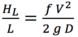 |
(1) |
where HL is the head loss (m), L is the length of pipe under consideration (m), f is the friction factor (dimensionless), V is the velocity of water (m/s), g is the gravitational acceleration (9.81 m/s2) and D is the internal diameter of pipe (m).
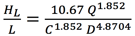 |
(2) |
where HL is the head loss (m), L is the length of pipe under consideration (m), Q is the volume of flow of water (m3/s), C is the Hazen-Williams roughness constant and D is the internal diameter of pipe (m).
HW equation mentioned above is found in literature in various forms depending upon the units of measurement being used for the study (Jamil, 2015), though the variables involved remain the same. It is observed that for smaller pipe diameters and lower water flows, there is only a slight discrepancy in results obtained from equations (1) and (2) when used under identical conditions, but this becomes more significant for larger diameters and higher flows. One of the reasons for this discrepancy is the roughness coefficient involved in both equations. In HW equation a single roughness coefficient is used for all diameters of a single pipe material without considering fluid temperature, but in DW equation the friction factor varies with the flow conditions including pipe diameter, flowrate, fluid temperature, etc. (Kamand, 1988). Hence it becomes necessary for the manufacturer to test the performance of pipes by using both the equations to satisfy their clients that the manufactured product conforms to all applicable codes and standards. However, the frequency of use of both equations varies a lot. As mentioned by Rossman (2000), HW equation was developed only for water and is applicable for a pipe flowing full with turbulent flow, whereas the DW equation is applicable for all flow regimes and can be used for any type of liquid. However HW equation is quite easy to use as compared to the other one because all the parameters involved are easily available in the literature (Liou, 1998). Calculating head loss in pipes by using DW equation is relatively difficult because it involves separate calculation of the friction factor which is not simple. Friction factor is function of roughness height, pipe diameter, and flow. It is also dependent on Reynold’s Number (Eq. (3)) that further depends on density and dynamic viscosity which are functions of the temperature of the fluid.
| (3) |
where Re is the Reynold’s Number (dimensionless), ρ is the density of water at a specific temperature (kg/m3), V is the velocity of water (m/s), D is the diameter of pipe (m) and µ is defined as the dynamic viscosity of water at a specified temperature (kg/ms).
Hence, head loss estimation by DW formula needs a lot of additional data which varies with temperature of water. If such data is not used correctly or in case of unavailability, may result in a significant error. This becomes a matter of concern for the manufactures of hot water pipes when they have limited access to literature and research data.
Determining f for a laminar flow for which Re < 2000, is easy and is given by Eq. (4) which is also known as Hagen-Poiseuille’s equation (Allen, 1996).
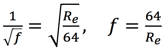 |
(4) |
where f is the friction factor (dimensionless) and Re is the Reynold’s Number (dimensionless). However, for the transitional and turbulent flows for which Re ≥ 2000, friction factor is the main issue in the DW equation. Colebrook (1939) proposed an implicit equation (Eq. 5) for the solution of f, which is known as Colebrook-White equation that is recognized to be the most accurate for the solution of Darcy’s friction factor (Liou, 1998).
| (5) |
where f is the friction factor (dimensionless), ε is the roughness height, D is the diameter of the pipe (m) and Re is the Reynold’s Number (dimensionless).
In 1944, Moody (1944) presented the charts for the approximation of friction factor for all flow regimes based on CW equation. His work was completely based on experiments and he did extensive work to develop those charts. Moody’s chart is widely accepted as the best representation of Colebrook-White (CW) equation for the calculation of friction factor and is considered to be famous and most useful in fluid mechanics (White, 2008).
However, the major issue with CW equation is that it is implicit in terms of f. An iterative solution is required for this equation to determine the value of f which becomes complicated. Even though various studies are available exclusively for the indirect solution of CW equation, no direct solution is available owing to its implicit nature. Researchers used computer applications (Yildirim, 2009; Brkić, 2011b and Shaikh et al., 2015), mathematical techniques (Sonnad, 2006; Travis and Mays, 2007; Clamond, 2009 and Brkić, 2011a) and manual calculations (Rollmann, 2015) for the closest possible solution of CW equation. Bagarello et al. (1995) performed experiments on small plastic diameter pipes to calculate head losses by using DW equation where he assumed f to be the approximation provide by Blasius equation shown below which was proposed by Blasius in 1913.
| (6) |
where c and m are the coefficients whose empirical formulae were proposed by Bagarello et al. (1997)
| (7) |
and
| (8) |
Although the experimental results obtained by Bagarello et al. corresponds to the one obtained by using Blasius equation, it was learnt that the experiments were limited for only small diameter pipes (DN 16, DN 20 and DN 25) having a range of Reynold’s numbers from 3,000 to 36,000. On the other hand, this article deals with five different diameter plastic pipes having Reynold’s numbers of 6,000 to 360,000 — 10 times larger than those of the research done by Bagarello et al. Also the Blasius’s approximation of the factor f is older than the CW equation which was proposed in 1939 and considered to be the most reliable approximation of friction factor in DW equation. Hence the results obtained by using Blasius approximation are not considered to be carried forward for this research.
Furthermore, Valiantzas (2005) provided a modified form of HW and DW equations for irrigation pipes which are limited to cold water supply only. Although the modified equations were further corrected by the original author (Valiantzas, 2007) followed by the published discussion article (Provenzano et al., 2007). However it still did not discuss the supply of hot water as the original research was meant for irrigation water supply and hot water supply was out of the scope of the research.
Brkić (2016) and Huang et al. (2013) did extensive experimental works on determining the value of friction factor for various flow conditions separately. However, the literature reveals that there is no direct and reliable solution for the CW equation. For instance, Mohsenabadi (2014) compared the results of almost 30 available explicit equations for the solution of CW equation, and concluded that all equations had their limitations and had significant differences in their results. Hence none of the approximate solution of CW could be considered reliable.
To address this issue, it was considered better to use an iterative technique, which is the focus of this article. The functionality of Microsoft Excel was exploited for the proposed iterative method. A tedious exercise was done to complete the iteration for all 420 values for DW equation, which yielded good results and precise values of f for each model under each flow condition. It is also obvious from the literature that there is a lack of a relationship between HW and DW equations. Such a relationship would be very useful for manufacturers and designers for the mutual conversion of head loss values obtained by these equations. As plastic pipes are now very common for hot and cold water applications in buildings as well as infrastructure projects due to the ease of installation, jointing, repair and handling, plastic pipes are replacing metallic pipes. Also researchers are now keen to develop and study the properties of new plastic pipe materials as well (Jamil, 2018). Accordingly, the present work is aimed to develop a correlation between HW and DW equations for plastic pipes of diameters from 15 mm to 50 mm, by considering full flow of water in a temperature range of 20-60º C.
Methodology
The HW constant and roughness height in DW equation for plastic pipes were kept as 150 (Rossman, 2000) and 0.0015 mm (White, 2008) respectively, as available in the literature. The results obtained by DW and HW equations were compared under identical conditions. Head loss per unit length was calculated for various scenarios.
As already mentioned, the value of f in DW equation depends on Re which is a function of density and dynamic viscosity, which themselves are temperature-dependent. As shown in Fig.1, five hydraulic models were developed by considering minimum temperature of cold water as 20o C and maximum temperature of hot water as 60o C (Church, 1979), pipe diameters ranging from 15 mm to 50 mm, and flow rates ranging from 0.25 lps (liters per second) to 2 lps, as commonly adopted for buildings.
The values for the density and dynamic viscosity of water were taken with respect to the selected temperatures of water (White, 2008). This methodology generated 42 values per model for each equation, amounting to a total of 420 values for both equations from five models, which were then used for the analysis. The input parameters for the models are summarized in Table 1.
The head loss was estimated for each model for all flowrates and pipe diameters considered. The Re values calculated for the above mentioned flow conditions ranged from 6,000 to 360,000, which indicated that the flow was turbulent in each model. This satisfies the condition for the validity of both DW and HW equations, justifying a common base to compare the results of both equations.
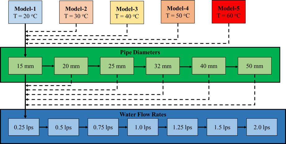
Figure 1: Schematic representation of research work flow
Results and Discussion
Correlation Coefficient
One of the techniques of Inferential Statistics in mathematics while comparing two variables is to determine whether a relationship between them exists or not. Accordingly, prior to developing an empirical relation between DW and HW equations, a correlation coefficient between them was measured by using the formula (Bluman, 2009):
| (9) |
By using the values of head loss obtained from the developed models, the Correlation Coefficient was estimated to be 0.999, which indicates a strong positive relation between the two equations.
Effect of Temperature on Head Loss and Reynold Number
An initial analysis was performed to observe the effect of temperature on the calculated head losses. The values for an average pipe diameter of 25 mm were taken and then plotted against the flowrates for all models, mentioned in Table 1, separately.
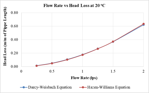
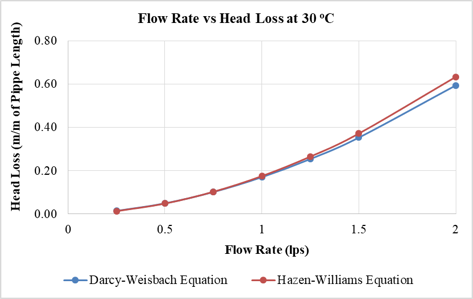
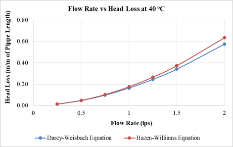
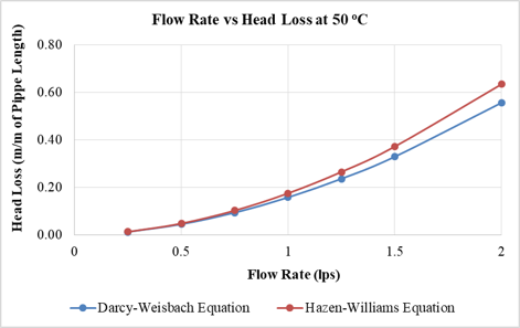
Fig. 2 shows the relationship of head loss obtained by using both DW and HW equations against a specified temperature for a pipe diameter of 25 mm. It can be observed that as the temperature increases the difference between the head losses obtained by both equations also increases. But in buildings the temperature of water supplied does not increase above 60º C, so there is no need to consider higher temperatures. Moreover it is noted that the pattern of increase in head loss with the increase in flow rate remains the same for all models.
Another plot was created to validate the calculated Re values for all the five models described in Fig. 1. The graph shows the variation in Reynold’s Number with the increase in the flow rate as well as increase in temperature of water. The range of Reynold’s Number, at which this research has been completed, can be observed through this plot shown in Fig. 3. It can be seen that the value of Re increases with the increase in temperature and flow rate of water in a typical pattern for all five models, proving that the calculated values used for the research are justified.
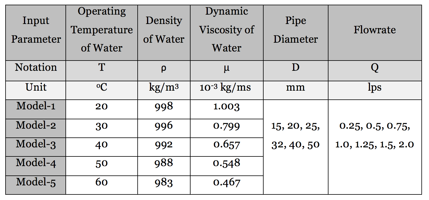
Table 1: Input parameters for the hydraulic models.
(Below) Figure 2: Flow Rate vs Head Loss Plots for 25 mm dia. pipe at (a) 20o C, (b) 30o C, (c) 40o C, (d) 50o C and (e) 60o C
a.
b.
c.
d.
e.
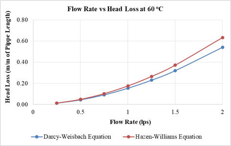
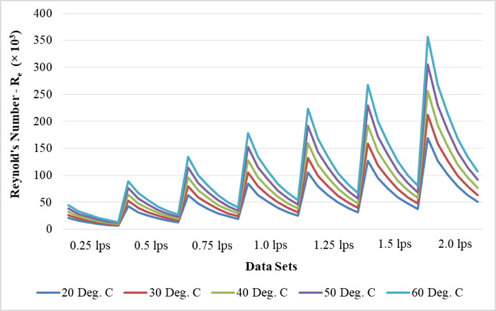
Figure 3: Variation in Reynold’s Number against varying temperature and flow rate
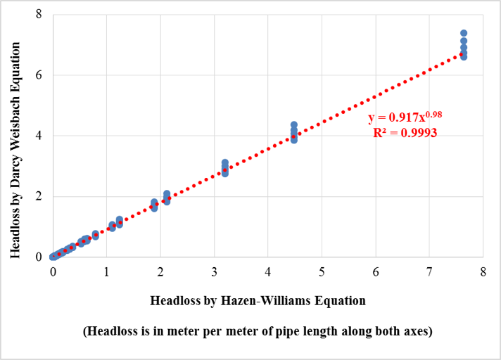
Figure 4: Darcy-Weisbach vs Hazen-Williams Equation
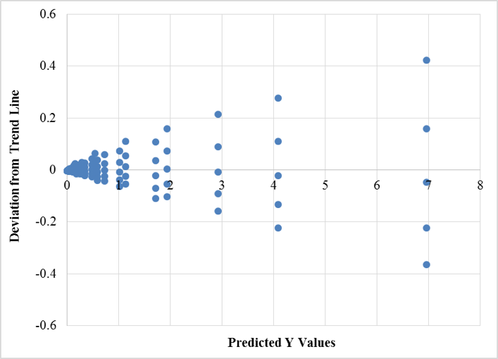
Figure 5: Residual plot for trendline
Relation between HW and DW Equations
The major part of the data analysis is to develop a relation between both the renowned equations. Hence, the values of head loss per unit length of a plastic pipe obtained from all the five models were plotted as shown in Fig. 4. It is observed that the values are very precise and close to each other, and they follow a certain pattern. A trend line was plotted for the scatter plot whose equation came out to be:
| (10) |
Eq. (10) can be re-written in terms of the variables under study as:
| (11) |
where Dw and Hw are the head loss in meters per meter (m/m) of the plastic pipe, obtained by DW and HW equations respectively. Eq. (11) is the empirical relationship intended to develop in the current study.
The R2 value for the trend line was found to be 0.9993, which indicates excellent accuracy in statistical terms. This is further substantiated by the residual plots (Fig. 5) that show that only 2 out of the 420 values deviate with an average of ±0.3 units from the trend line. These values were traced to be for 50 mm diameter pipe. Though the deviation is negligible in this case, it can be deduced that with the increase in pipe diameter and flowrate, the head loss value would deviate more from the trend line. Hence the present empirical relationship should be considered valid to a maximum of 50 mm diameter of plastic pipes.
Furthermore, the calculated values of f and Re were plotted as in Fig. 6, which shows a perfect fit of the Moody’s chart. This shows that the manual calculations performed for the DW equation are good and perfectly reliable to be used for developing correlation with HW equation.
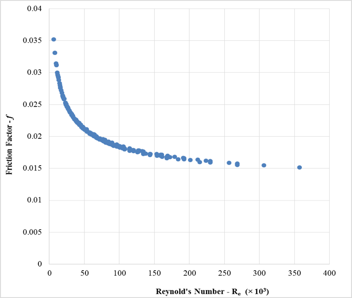
Figure 6: Reynold’s Number plotted against Friction Factor
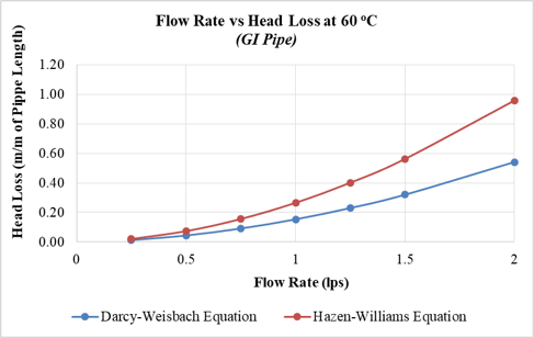
(Below) Figure R1: Flow Rate vs Head Loss plots for 25 mm dia. GI pipe at (a) 20º C and (b) 60º C
a.
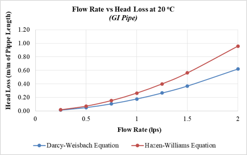
b.
Conclusion
An empirical relation between Darcy-Weisbach (DW) and Hazen-Williams (HW) equation has been developed, for cold and hot water flows through plastic pipes. The data for establishing the proposed relationship were obtained from hydraulic models developed for water temperatures ranging from 20º C to 60º C, pipe diameters from 15 mm to 50 mm, and volume flowrates from 0.25 lps to 2 lps. The unique feature of this relationship is that it can be used to determine the head loss obtained by DW equation directly without calculating the friction factor and Reynolds number when the corresponding value by HW equation for similar flow parameters is available. This feature makes the task easy for pipe manufacturers and related industry. The relation is valid for hot and cold water plastic pipes within the diameter range 15 mm – 50 mm and water temperature 20º C – 60º C. However, for larger flows and larger diameters, the values are found to significantly deviate from the trend line, which marks the limit of the proposed correlation.
Discussion with Reviewers
Reviewer: Is the developed relation valid in extreme conditions e.g. cold flow in hot weather and similarly hot flow in cold weather?
Authors: Steel pipes in general have a very high rate of thermal conductivity, and according to a few studies, the temperature of the external surface of a metallic pipe is the same as that of the water flowing inside it. But on the other hand, the thermal conductivity of plastic pipes considered for this research is almost 50-60% less than that of steel pipes (Corzan, 2018). As an example, during extreme cold weather the water flowing inside a plastic pipe at 50-60º C may fall to 35-45º C. Similarly, during extreme hot weather the temperature of water inside the pipes may jump to 30-40º C from 20-25º C. It is seen that, the change in the temperature of water caused by the extreme weather conditions remains within the temperature range considered for this study. Moreover, as a protective measure, water supply pipes are provided with thermal insulations throughout their lengths to deny any effect of external temperature on the temperature of water inside the pipe resulting in further decrease in the difference in temperature. Hence it can be said with confidence that the developed relation is equally valid for extreme weather conditions.
Reviewer: How much difference in results is expected in other types of pipes?
Authors: For other materials of water supply pipes the difference in the calculated head loss values is found to be huge. For instance, Galvanized Iron (GI) pipe was considered for comparison having a Hazen-William Constant of 120. For a 25 mm diameter GI pipe having water flowing at 2 lps and at 20º C, the difference in head loss jumped to 55% from only 1.5% as shown in Fig. R1a. Similarly, for a 25 mm diameter GI pipe having water flowing at 2 lps and at 60º C, the difference also increased to 78% from 17% as shown in Fig. R1b. Figures developed for GI pipe, mentioned below, can be viewed in conjunction with Fig. 2 to notice a significant difference. The developed relation is only valid for plastic pipes which are more commonly used and have a lot of benefits over other pipe materials. The research can be extended at later stage to study the effects caused by other pipe materials.
References
Allen RG (1996) Relating the Hazen-Williams and Darcy-Weisbach Friction Loss Equations for Pressurized Irrigation, Applied Engineering in Agriculture, American Society of Agricultural Engineering, 12 (6): 685-693
Bagarello V, Ferro V, Provenzano G, Pumo D (1995) Experimental Study on Flow-Resistance Law for Small Diameter Plastic Pipes, Journal of Irrigation and Drainage Engineering, 121 (5): 313-316
Bagarello V, Ferro V, Provenzano G, Pumo D (1997) Evaluating Pressure Losses in Drip-Irrigation Lines, Journal of Irrigation and Drainage Engineering, 123 (1): 1-7
Bluman AG (2009) Elementary Statistics: A Step by Step Approach, McGraw-Hill, New York, ISBN 978–0–07–353497–8
Brkić D (2011a) An Explicit Approximation of Colebrook’s Equation for Fluid Flow Friction Factor, Petroleum Science and Technology, 29:15, 1596-1602
Brkić D (2016) A note on explicit approximations to Colebrook’s friction factor in rough pipes under highly turbulent cases, International Journal of Heat and Mass Transfer, 93 (2016): 513–515
Brkić D (2011b) Review of explicit approximations to the Colebrook relation for flow friction, Journal of Petroleum Science and Engineering, 77 (2011): 34–48
Churh JC (1979) Practical Plumbing Design Guide, McGraw Hill Book Company, ISBN 0-07-010832-3
Colebrook CF (1939) Turbulent Flow in Pipes with Particular Reference to the Transition Region between the Smooth and Rough Pipe Laws, Journal of The Institution of Civil Engineers, 11 (4): 133–156
Corzan (2018) Corzan Piping System Thermal Conductivity, https://www.corzan.com/en-us/piping-systems/specification/thermal-conductivity
Huang K, Wana JW, Chen CX, Li YQ, Mao DF, Zhang MY (2013) Experimental investigation on friction factor in pipes with large roughness, Experimental Thermal and Fluid Science, 50 (2013): 147–153
Jamil R (2015) Estimation of Sediment Deposition at Nausehri Reservoir by Multiple Linear Regression and Assessment of its Effects on Reservoir Life and Power Generation Capacity, International Journal of Advanced Thermofluid Research 1 (2): 46-59
Jamil R (2018) Performance of a New Pipe Material UHMWPE against Disinfectant Decay in Water Distribution Networks, Clean Technologies and Environmental Policy, 20 (6): 1287-1296
Kamand FZ (1988) Hydraulic Friction Factors for Pipe Flow, Journal of Irrigation and Drainage Engineering, 114 (2): 311-323
Liou CP (1998) Limitation and Proper Use of the Hazem-Williams Equation, Journal of Hydrauic Engineering, 124 (9): 951-954
Microsoft Product Support (2017) https://support.office.com/en-us/article/Change-formula-recalcula
tion-iteration-or-precision-73fc7dac-91cf-4d36-86e8-67124f6bcce4, Visited Nov 1, 2017
Mohsenabadi SK, Biglari MR, Moharrampour M (2014) Comparison of Explicit Relations of Darcy Friction Measurement with Colebrook-White Equation, Applied Mathematics in Engineering, Management and Technology, 2(4): 570-578
Moody LF (1944) Friction Factors for Pipe Flow, The American Society of Mechanical Engineers, 66 (8): 671–684
Provenzano G, Salvador GP, Bralts VF (2007) Discussion of “Modified Hazen–Williams and Darcy Weisbach Equations for Friction and Local Head Losses along IrrigationLaterals” by John D. Valiantzas, Journal of Irrigation and Drainage Engineering, 133 (4): 417-420
Rollmann P, Spindler K (2015) Explicit representation of the implicit Colebrook–White equation, Case Studies in Thermal Engineering, 5 (2015): 41–47
Rossman LA (2000) EPANET 2 User’s Manual, Water Supply and Water Resources Division, National Risk Management Research Laboratory, USEPA, Cincinnati OH
Shaikh MM, Massan S, Wagan AI (2015) A new explicit approximation to Colebrook’s friction factor in rough pipes under highly turbulent cases, International Journal of Heat and Mass Transfer, 88 (2015) 538–543
Sonnad JR, Goudar CT (2006) Turbulent Flow Friction Factor Calculation Using a Mathematically Exact Alternative to the Colebrook–White Equation, Journal of Hydraulic Engineering, 132 (8): 863-867
Travis QB, Mays LW (2007) Relationship between Hazen–William and Colebrook–White Roughness Values, Journal of Hydraulic Engineering, 133 (11): 1270-1273
Valiantzas JD (2005) Modified Hazen–Williams and Darcy–Weisbach Equations for Friction and Local Head Losses along Irrigation Laterals, Journal of Irrigation and Drainage Engineering, 131 (4): 342-350
Valiantzas JD (2007) Closure to “Modified Hazen–Williams and Darcy–Weisbach Equations for Friction and Local Head Losses along Irrigation Laterals” by John D. Valiantzas, Journal of Irrigation and Drainage Engineering, 133 (4): 420-421
White FM (2008) Fluid Mechanics, 6th Edition, McGraw-Hill Companies, Inc., New York, ISBN 978-0-07-064848-7
Yildirim G (2009) Computer-based analysis of explicit approximations to the implicit Colebrook–White equation in turbulent flow friction factor calculation, Advances in Engineering Software, 40 (2009) 1183–1190