Plant Electro-tropism

Author: Ramthun AD, 116 Standard Ave., Winsted, CT 06098,

(This paper was developed on the author’s own time and his expense and is not affiliated with any organization.)

Received November 22, 2015; Revised July 24, 2016; Accepted July 26, 2016; Published March 13, 2017;

Available Online March 14, 2017.

DOI: 10.14294/WATER.2016.6

Hypothesis

Electric forces on and within the mature sprout system of woody plants have the strength to define the plant’s growth, direction, and shape. Each branch and plant also electrically influences the shape and direction of neighboring branches and plants.

Abstract

This paper has transient voltage recordings of 1) Aspen (populus grandidentata), 2) Blue Spruce, (picea pungens), 3) Sugar Maple (acer saccharum), and 4) Corn (zea maize). The recordings show that large numbers electrons are flowing upwards on and in woody plants (trees). These electrons cover the plant and are proposed to create an electron cloud within the plant’s physical space. EZ water ions are proposed to collect inside the branch tips. The EZ water ions, electrons, and the earth’s electric field ions are used to calculate local bud system forces. These forces as calculated are pro-posed to be strong enough to direct the tree branches to be three dimensional (3d) solid copies of electric field “lines of force” as it grows.

A corn plant experiment shows the electron source is coming from outside the plant. An additional experiment shows a corn plant is moved by a horizontal electric field.

Keywords

Voltage, amperage, resistance, charge, capacitance, polarity, electron, Coulomb force, electric field, electric field force, electric field lines of force, plant electro-tropism, EZ water, electron cloud, restoring force.

Introduction:

The purpose of this paper is to help anyone observing plants to recognize and understand the electrical forces and lines of electrical force I believe define the shape of all woody plants.

In 1999, I became intrigued that plants appeared to follow the same rules as Electric Field Lines of Force in Figure 2 below. During the surveying of these lines of force using Voltage Circles in Figure 1 below, I learned that these lines of force repulsed each other and are a way to visualize the direction of electricity in an electric field continuum. These electric lines of force are invisible and undetectable by normal senses.

The electrical recordings and calculations of electric forces in this paper quantify electro-tropism and explain why woody plants grow away from the earth and why they grow away from each other.

This paper is based on observation, recorded evidence, electric force equations, calculations, experiments and conceptual drawings.

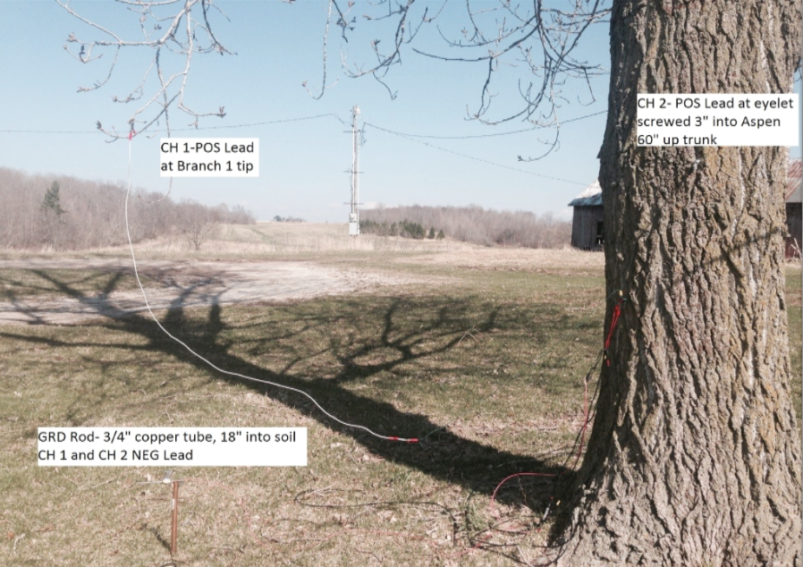
Transient recordings were taken on a large Aspen tree, a small Blue Spruce tree, a Sugar Maple tree, and a small corn plant.

The main test equipment used was a Velleman PCSGU250 2 channel oscilloscope, a Dell laptop, 100’ coaxial cables, coaxial test leads, and ground rod.

The plant voltage recordings in Appendix B, C, D, and E are all similar and consistent.

Phototropism and geotropism are well documented explanations for plant leaves and soft tissue growth direction and shape.

In this paper, electro-tropism means the plants woody sprout reaction to both internal and external electric fields and electric forces. See Appendix M-P for electric force calculations.

The electro-tropism electric model in this paper gives a fundamental mechanism and explanation for plants growth, direction and shape.

The term ions, protons, hydronium ions in this paper all mean positively charged particles.

The term electrons in this paper also means negatively charged particles.

The term “electron cloud” is used in many places throughout this paper. The EZ Water in a tree trunk separates protons and electrons on a continuous basis. These charges may or may not be permanently separated. The negative voltages shown in Appendix B-E are created by excess electrons and are likely partially from EZ Water, but also could be from the negatively charged earth and have a solar source.

There is evidence that an electron cloud with a frequency property similar to plasma exists within large trees. This plasma frequency property evidence is FM satellite radio interference ⁴³ (mid page) and GPS satellite signal interference near or under trees.

Both of these radio wave interferences have also been my observation. After purchasing a new car with satellite radio, my wife and I went on a fall color tour drive. We both noticed the radio cutting out when passing beneath large trees.

At my job, we do many survey grade GPS surveys. The base station receives GPS satellites signals and is always set up in an open area to best receive signals. However, the rover (data collector) also receives GPS satellite signals, and often loses signal when taking survey shots near large trees.

Electro-tropism provides a simple explanation why branches, and woody plants in close proximity grow away from each other.

Corn plant recordings of roots dipped in and out of water show negative voltages in the stem caused by dipping the roots in water. This electron source is thus coming from outside the plant.

A corn plant experiment shows a 10 volt/inch horizontal electric field deflecting and eventually killing the corn plant.

Vector cross product magnetic forces are exerted on the flowing electrons in the plants trunk and branches by the Earth’s magnetic field (similar to a sideways force exerted by a magnetic field on a current in a wire).

Magnetic force vector calculations and discussion are beyond the scope of this paper.

Tropism Discussion

Plants are a complex “system” involving chemical, mechanical, hydraulic, and electrical systems.

Current plant directional tropisms are Chemotropism, Gravitropism, Hydro-tropism, Heliotropism, Phototropism, Thermotropism, and Thigmotropism. (Wikipedia⁴)

Two other plant tropisms for nastic movements are non-directional, Nyctinasty and Thigmonasty. (Wikipedia)

None of the current plant tropisms consider electric force vectors.

Phototropism is the most easily observed of tropisms when leafy plants respond to light. None of the phototropism models or mechanisms I’m aware of, consider the possibility that electric forces could be causing the phototropic effect, leaves are covered with electrons (See Appendix E – Figure 21) and sunlight is an electromagnetic wave.

All of these plant tropisms have two things in common. First, they all use local differential cell growth argued to be caused by auxin to explain the change in the plant growth direction. Second, none of them consider electric force vectors to explain the plant change in growth or direction.

None of the tropisms other than Electrotropism have the ability to quantify the overall plant system vector forces. Electric vector forces such as needle to needle forces, branch to branch forces, or plant to plant forces have been overlooked in the current plant tropisms.

Why aren’t electric forces on or within the plant considered?

Possibly the main reason the electric effects on plants has been missed is not understanding what is being seen.

The prevailing argument is that all plants are “reaching for sunlight.” While it is true that soft, leafy plants dominated by phototropism reach for sunlight, woody plants ignore sunlight direction and grow directly perpendicular to the earth at all latitudes.

Geotropism is the prevailing argument for plants growing away from the earth, I would argue that the electric repulsive forces between plant electrons and earth electrons are an integral reason plants grow away from the negatively charged earth. Additionally when a plant is “knocked down” by physical forces, the repulsive electrical forces between plant electrons and earth electrons greatly increases to push the plant back to an upright position. While auxin directs cell elongation and growth to assist the plant to right itself, I believe the force which causes cell elongation is an internal repulsive electrical force or “restoration force” called F_e ³⁸.

Geotropism and phototropism both fail to explain how neighboring woody plants or plant branches, or blue spruce needles repulse each other.

Electricity on and within the plant is not evident by normal human perception because it is normally below 1 volt. Electricity is also not likely a normal field of study for plant biologists, who focus on chemistry as evident by past and current research. Even within the physical sciences, electricity is often poorly understood as evident by astronomers focusing on gravity, to explain the universe, while mostly ignoring electric forces.

Auxin or Indole-3-acetic acid (IAA) is the most common, naturally-occurring, plant hormone of the auxin class. Auxin is well proven to be directly involved with plant growth and cell elongation.

From my own electrical measurements on plants, it is evident that they are covered with an extreme number of electrons. Gently setting the voltmeter positive lead on a blue spruce branch, results in a flurry of negative voltage readings of approximately 1.0 volt with reference to ground several feet away.

Not only are there many, many electrons on the plant exterior as evidenced in Appendix B-E, but there is continuous charge separation in the plant moisture due to the recently discovered Exclusion Zone or fourth phase of water caused by infrared energy1 (Pollack, GH, 2012, Fourth Phase of Water, Ebner and Sons, Seattle, WA, Chapter 6).

For abundant visual evidence of electricity’s effect on plants, it is a main contention in this paper, that all parts of woody plants display “electric field lines of force” if not distorted by mechanical forces such as gravity, wind, snow, ice, etc.

Appendix A 1999 Electric Field diagram was derived using a large number of voltage circles to draw the large scale electric field lines of force. See Figures 1 and 2 below. Similar electric field lines of force, in my opinion are readily evident in woody plants. Young maple trees without leaves are very good examples. Branches at or near the top of trees also show electric field lines of force most clearly.

In leafy plants dominated by phototropism, it is difficult to see electric field lines of force. It is also difficult to see in woody plants with physical damage, or in old trees.

Currently, the effect of electro-tropism has not been shown on a plant scale, but in Wikipedia it refers to the control of growth in cells and pollen tubes. See below.

Electrotropism [20] is a kind of tropism which results in growth or migration of an organism, usually a cell, in response to an exogenous electric field. By imposing an exogenous electric field, or modifying an endogenous one, a cell or a group of cells can greatly redirect their growth. Pollen tubes, for instance, align their polar growth with respect to an exogenous electric field.[3] Electric fields have also been shown to act as directional signals in the repair and regeneration of wounded tissue.[4] Wikipedia.

Symbol	name	value	SI unit	Abbreviation
E	electric field	–	newton/coulomb	nt/coul
F	force	–	newton	nt
q₀	scalar charge	–	coulomb	coul
π	pi	3.1416	–	–
є₀	permittivity constant	8.85418 x 10^-12	coul² /nt-m²	–
к	dielectric constant -water	78	–	–
C	capacitance	–	farad	–
1/4πє₀	–	9.0 x 10⁹	nt-m² /coul²	–
m	meter	–	meter	m
cm	centimeter	–	centimeter	cm
r	distance between charges	–	meter	m
V	voltage	–	volt	V
I	amperage	–	ampere	amp
Ω	resistance	–	ohm	R
e	electron	1.6 x 10^-19	coulomb	coul

Table 1. Symbols and Abbreviations

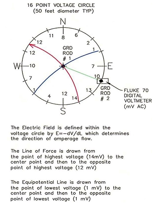
$C:\Users\Arde\Pictures\WJ pictures\Voltage Circle Diagram.jpg$
Figure 1.

16 Point Voltage Circle Procedure.

Orient to N-S.

Use tape measure to find center.

Place center Grd Rod # 1.

Measure voltage between Grd Rod #1 and Grd Rod #2 at 16 equally spaced points around circle.

Draw Electric Field Line of Force from highest voltage to center to highest voltage on opposite side of circle.

Draw equipotential line from lowest voltage on circle to center to lowest voltage on opposite side of circle.

Repeat procedure for new Voltage Circle.

Electric Field Lines of Force Lessons Learned

The Lines of Force in Figure 2 of Appendix A:

Repulse each other.
Are curved and flowing around a blocking electric field not shown on the right.
Change direction only because of another electrical influence.
Changing soil type from sand to clay (about 100’ up on Diagram 2 below) had no noticeable effect on the Lines of Force direction.
Will flow in a straight in the absence of other electrical forces.
Will flow in a straight line through electrical forces equal on both sides.
Gave me the idea that plants follow the same rules.

Voltage Recording and Resistance Reading Methods and Procedure

Test equipment lessons learned

PC based oscilloscope channels are not independent on this oscilloscope model.

Poor bonding results in bad data.

Branch resistance readings require a fresh multi-meter battery.

Care was taken to ensure polarity integrity using red and black tape to mark the plugs.

Resistance readings were also done to verify polarity integrity. ID tags were used on the branches.

To prevent interference, the recordings were done with the laptop on battery power, as well as lights and shop equipment shut off.

Alligator clips with conductive paste were firmly squeezed on to branch for voltage readings.

Both alligator clips and special copper clips with conductive paste were used for voltage and resistance recordings.

Resistance Readings Method

Copper spring clips shown below have stainless steel screws with sharp points used to perform branch resistance readings. The sharp points penetrated the branch bark, especially the smaller branch tip area. Limited readings were taken because the sharp points damaged the bark.

May 24, 2014 Results: all readings are about 1” from the branch tip to 18” along branch. All branches were pre-wetted with tap water or conductive gel.

Results:

Aspen Branch 1 = 1.9 MΩ,

Aspen Branch 2 = 2.1 MΩ

Blue spruce Br 5 = 2.8 MΩ,

Blue spruce Br 6 = 0.9 MΩ

Blue spruce Br 7 = 1.5 MΩ,

Blue spruce Br 8 = 1.3 MΩ

Blue spruce Br 9 = 1.8 MΩ,

40’ maple Br 8 = 0.5 MΩ

Average ohms reading = 1.6 MΩ

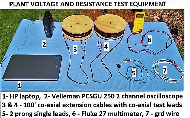
$C:\Users\Arde\Pictures\WJ pictures\Test Equipment.jpg$

Picture 1. Voltage and resistance reading and recording test equipment.

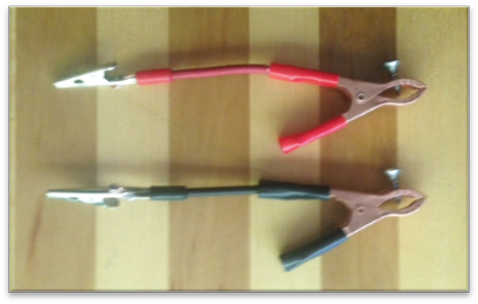
$C:\Users\Arde\Pictures\Plant pictures\Clips with SS screw.JPG$
Picture 2. Small copper branch clamps with stainless steel screws.

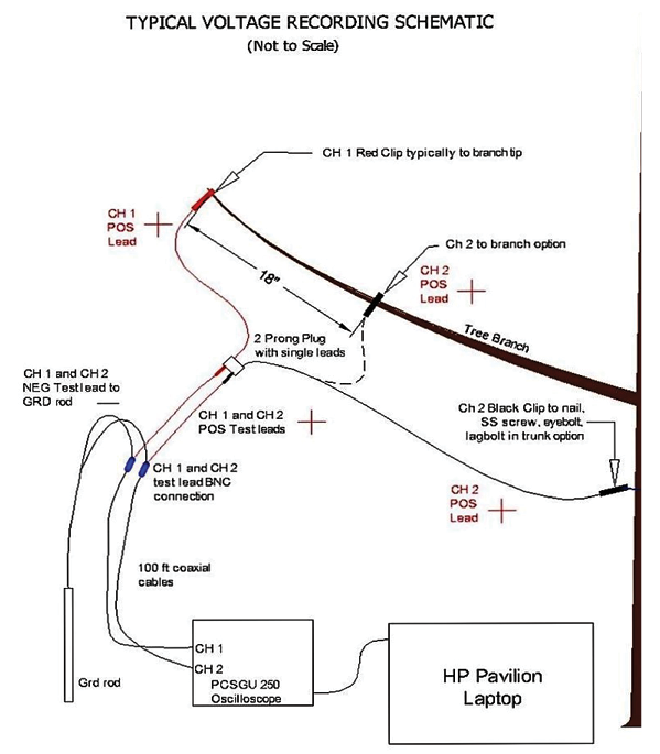
$C:\Users\Arde\Pictures\WJ pictures\Schematic.jpg$

Picture 3. Typical Electrical Recording Test Schematic. See Tektronix Application Note – Fundamentals of Floating Measurements and Isolated Input Oscilloscopes. “A minus B” Measeurements.²¹

Voltage Recording Discussion

The voltage recordings (See Appendix B, C, D, E) show consistency with time and across plant species (an exception is Spruce Recording 1 which shows a higher voltage mid trunk than at the trunk base). It should be noted that this spruce recording POS lead pin was only 2” above the ground surface. The other trunk recordings were done farther up the trunk.

All recordings show the largest negative voltage (analogous to water pressure) is within the tree trunk. The branches near the trunk have less negative voltage than the trunk, and the branch tips farthest from the trunk have the least negative voltage. Therefore the negatively charged particles (assumed to be electrons) are flowing up the trunk and outwards to the branch tips.

The voltage recordings are repeatable. More channels on the oscilloscope would better quantify how many electrons are flowing in each minor branch.

What is the Charge Polarity on PCSGU 250 Recordings?

Assume negative charge is an “excess of electrons.

Assume positive charge is a “deficit” of electrons.

Assume a battery has excess electrons at the negative terminal and deficit electrons at the positive terminal.

Positive voltmeter lead (red) to positive battery terminal and negative voltmeter lead (black) to negative battery terminal gives a positive voltage reading.

Positive voltmeter lead to negative battery terminal and negative voltmeter lead to positive battery terminal gives a negative voltage reading.

Therefore, similar to a battery reading, a voltage recording line below the Reference (Ref) line is a negative voltage reading on the PCSGU 250 Graph which indicates an excess of electrons, and a negative charge polarity.

Hypothetical Two Meter Tree Electric Model Overview

Tree height and branch lengthening begins with a bud. Tree height growth is caused by the apical meristem whose cells divide and elongate at the base of the bud to create upward growth in trees with a dominant crown tip.²⁸

The bud or tip of the branch is the focal point of the force calculations below. Branch voltage recordings and branch resistance readings lead to an amperage calculation. Bud capacitance is calculated, then bud charge. Tip moisture acting as a dielectric³⁰ between bud plates is the reason charge accumulates inside the tip. Protonated EZ water flows to the tip and accumulates. For hundreds of years water has been known to hold a charge.

(See Leyden’s Jar.²⁹ )

Water will hold a static charge inside the branch tips. EZ water produces ions and electrons wherever water is in the plant.

While the majority of wood in a tree is dead the entire tree is moist³¹ (See Table 4.1).

So a 100-lb tree with a 100% moisture con-tent is 50 lbs of wood and 50 lbs of water (wet basis). The water in the cam-bium is moving towards the branch tips and the water in the heartwood is less mobile because the dead cells are not well connected.

EZ water hydronium ions travel to and are trapped inside the bud. The ions attract electrons which are electrostatically held to the outside of the bud. These held electrons act as a block to incoming electrons flowing towards the bud. It is logical to assume the incoming electrons are forced off the branch just prior to the bud. As shown in Figure 26 below, the electrons around the bud form an electron cloud with a restoring force F_e³⁸.

In my opinion, the calculations in Appendix F-P are reasonable estimates of capacitance, charges at the tip, trunk, air, and forces. The resultant force calculations with and without the electron cloud shows that the electron cloud is key. The below model of a hypothetical tree models a branch tip and trunk of a 2 meter tall tree.

Electric Equations

Electric Equations and Ohm’s Law

F = (1/4πє₀) (q₁ x q₀)/r² Coulombs Law⁴ (Eq. 1)

E = F/q0 = (1/4πє₀) q/r² E= Force/test charge⁵(Eq. 2)

Note: Eq. 1 and Eq. 2 are equivalent for stationary charges.

V = IR Ohm’s Law⁶ (Eq. 3)

Note: Ohm’s law holds for metallic conductors. The resistance of moist wood will vary with the degree of water polarization.

I = q/sec Amperage = charge/second by definition⁷ (Eq. 4)

C = q/V Capacitance = charge/volt⁸ (Eq. 5)

C = к є₀ A /d Capacitance of parallel plate capacitor⁸ (Eq. 6)

C = к π є₀ l / ln (d/2a + (d²/4a² -1)^{^1/2}) Cap. parallel conductors, ³⁶(Eq. 7)

Amperage Flowing Towards Branch Tips

I = V/R Ohm’s Law (Eq. 3)

Assume: Aspen Branch average resistance R = 2 MΩ

From the Figure 14 Aspen Recording, V = -90 mV (-0.090 V), then

I=-0.090 V / 2,000,000 ohms = -4.5 x 10 ^-8 ampere (coul/sec)

Electrons/second

Elementary charge e = 1.60 x 10^-19 coulomb Halliday and Resnick Physics, App. A, pg. 45

By definition: 1 electron has 1 elementary charge, therefore;

Electrons/sec = 4.5 x 10 -8 coul/sec / 1.60 x 10 -19 coul/electron = 2.8 x 10 11 electrons/sec

Therefore: 280,000,000,000 electrons/second flow to the tip of each small Aspen branch

However this amperage flow is on the outside of a large tree branch.

What is going on inside the tip of the hypothetical 2 meter tree?

Charge Inside the Branch Tip

The below bud (tip) Picture 3 shows a tightly bound layered leaf system which I modeled using Eq. 6 to calculate the tip capacitance using plates in parallel. I dissected A _bud from a Laurel bush (Kalmia latifolia) and found several separate semi-spherical plates of different sizes. (Similar to the Sycamore bud below) The plates were very thin and each had two layers. Using graph paper I estimated the total leaf area (A) of 1.2 sq. inch (0.00077 m²). (I counted each leaf area from one layer not two layers). The thin plates show nature is optimizing capacitance and charge in my opinion.

Eq. 6, gives greater capacitance the thinner the gap between charged plates is. The gap between the two layers of each plate was extremely small and likely containing moisture acting as a dielectric.

Picture 3 and 4 below of terminal buds illustrates that charge in the tip will block incoming hydronium ions (protons) created in the trunk and branch EZ Water (see Figure 7 and 8 below).

A blocking charge in the terminal bud will force the secondary buds to emerge. The two secondary tips are directly opposite which is likely caused by protons repulsing each other. This is the basis of all branching in my opinion. When the protons flowrate in the water increases to a certain threshold, the repulsive force in the water forces branching to occur.

Q _{tip plate} = 2.3 • 10^-7 coulomb (protons inside tip), See Appendix F for capacitance and charge calculations.

The below Pictures 3 and 4 of terminal buds and two secondary buds illustrates the layers that make up the terminal bud and are the basis for the bud capacitance calculation in Appendix F.

The bud or tip often consists of a tightly wound group of young leaves. The edges of these leaves are also good charge concentration points.

The tip charges will continuously change and will vary by stage of bud growth, plant metabolic rate, and season. As an example, the water and proton flow will be greatly decreased during dormancy. I believe the very thin leaves in the tip are evidence that nature is optimizing the use of tip capacitance and charge to increase the branch competitiveness with other branches and other plants.

The protons inside the tip in Figure 26. Bud Local Charge System below and corresponding electrostatically attracted negative charges outside the tip are physically isolated from each other by the tips outer cells. When the plant is leafed out, some of the electrons will neutralize the protons (hydronium ions).

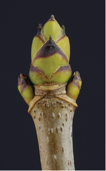
Picture 3. Sycamore bud³⁴

Picture 4. Maple buds³⁴

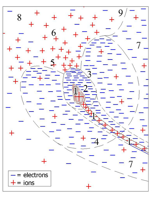
Figure 26. Bud Local Charge System (Not to scale)

In Figure 26 above, the numbers 1-9 mean;

Q _{tip plate} = 2.6 • 10^-7coulomb (protons inside tip) See Appendix F
Q _{tip net} = -5.2 • 10^-9 coulomb (2% of electrons outside tip) See Appendix H
Boundary of tip electrons, Q _{tip total electron} = -2.65 • 10^-7 coulomb, Appendix I
Force boundary between the tip electron cloud restoring force field and the tree electron cloud restoring force F_e. The tip electron cloud restoring force = the tree electron cloud restoring force. See Appendix J
“Hole” in the tip electron cloud caused by concentrated earth electric field ions neutralizing the concentrated electrons.
Concentrated earth electric field ions drawn in by Q _{tip total electron}.
Tree electron cloud field. See Appendix J
Earth Electric Field
The boundary between tree and earth electric fields. At this boundary, the number of electrons = the number of ions, therefore F_e = 0. The green dashed line in Figure 8 – Electron Flow Diagram also represents the “9” boundary.

Figure 26 Bud Local Charge System is an illustration showing both ions and electrons near the bud as an electron cloud with possible plasma properties. ²⁴

Electrons continue to flow towards the bud and are deflected away by the concentrated and static electrons around the bud. The PCSGU voltage recordings in Appendix B-E show the steady negative current flowing towards the buds.

Tree Trunk Layers

Tree Trunk Layers and Rings

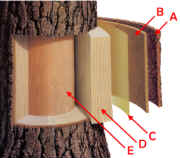
Figure 5. Trunk Layers 32
A = outer bark, B = inner bark, C = cambium, D = sapwood, E = heartwood

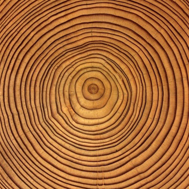
Figure 6. Tree Trunk Rings ³⁵

Appendix G shows the tree rings “early wood” (light colored part of ring) and “late wood” (dark colored part of ring. Large, water conveying vessels are shown in the early wood. The late wood thicker cell walls and does not convey water with long open vessels.

The trunk layers B, C, D and E in Figure 5 above all contain moisture.

The inner bark, or “phloem,” is pipeline through which food is passed to the rest of the tree. It lives for only a short time, then dies and turns to cork to become part of the protective outer bark.

The cambium cell layer is the growing part of the trunk. It annually produces new bark and new wood in response to hormones that pass down through the phloem with food from the leaves. These hormones, called “auxins,” stimulate growth in cells. Auxins are produced by leaf buds at the ends of branches as soon as they start growing in spring.

Sapwood is the tree’s pipeline for water moving up to the leaves. Sapwood is new wood. As newer rings of sapwood are laid down, inner cells lose their vitality and turn to heartwood.

Heartwood is the central, supporting pillar of the tree. Although dead, it will not decay or lose strength while the outer layers are intact. A composite of hollow, needlelike cellulose fibers bound together by a chemical glue called lignin, it is in many ways as strong as steel.

Since all the above layers contain either static or moving moisture, the entire tree trunk has increased capacitance because water has a high dielectric constant (78) and can hold a charge. See Leyden’s Jar.¹⁵

Assume the tree trunk rings contain vessels that can be modeled using parallel conductors as capacitors. Similar to the thin leaves in the tip, nature is optimizing the effect of charge using small diameter vessels. Both Eq. 6 and Eq. 7 calculate increased capacitance with thin layers using 1/d and 1/ln (d/2a + (d²/4a² -1)^{^1/2)} respectively. The smaller (d) the distance between vessels is and the smaller the difference between vessel radius (a) is the greater the capacitance.

The calculated charge inside the trunk is assumed negative because the trunk is continuously losing EZ water protons in water transported to the branch tips.

EZ Water and Trunk Charge

Figure 22 and Figure 23 in Appendix G show why tree rings vessels can be considered parallel conductor capacitors acting in pairs using Eq. 7. The early wood has large open cells which holds and transports more water than the darker small diameter late wood cells.

Figure 7 below shows EZ water producing a steady stream of protons inside of a hydrophilic tube. Figure 8 below verifies the same effect in plant xylem (sapwood). EZ water is energized primarily from infrared energy.¹ (The Fourth Phase of Water, Chapter 6, page 88, Chapter 7, page 119)

The trunk EZ water is continuously losing protons and leaving electrons behind. The hypothetical two meter tree trunk reaches a maximum negative charge = -2.0 • 10^-4 coulomb calculated in Appendix G.

Q_trunk = -2.0 • 10^-4 coulomb

Trunk charge apparently has two main energy sources. 1) Infrared energy, and 2) the electric field across the plant as shown in the right side of Figure 4 in Appendix G.

Having two steady sources of energy to charge water helps the charge in the trunk remain stable. During extreme cold, when infrared energy is weak, the plant electric field will keep the water charged.

Q_trunk / Q_tip plate = -2.0 • 10^-4 coul / 2.6 • 10^-7 coulomb = 769, trunk charge to tip ion charge ratio

Because the trunk loses protons to the buds continuously from EZ Water, the electrons inside the trunk outnumber the ions. These excess electrons create a radiating restoring force F_e inside the trunk and branches. I believe this F_e force causes tree ring growth and elongation in both the trunk and branches.

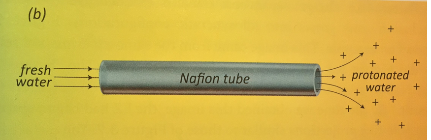
Figure 7. (Figure 5.4, Chapter 5 page 75) ¹

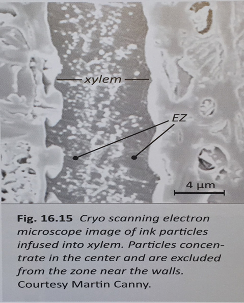
Figure 8. EZ Water in Xylem (page 300) ¹

Annual plant stems such as wheat, oats, or rye have hollow cylindrical stems. These hollow stems could be modeled using the equation for cylindrical capacitance:

C = к є₀ 2πl / ln (b/a) Capacitance of coaxial cylinder9

Resultant Force Discussion

Vector Force Calculations – No electron cloud, Appendix O and P

Coulomb force calculations were performed based on calculated bud charge, (Appendix F), and trunk capacitance and charge, (Appendix G) as shown in Appendix O and P. In my opinion, these calculations in Appendix O and P failed to give a reasonable model for Plant Electro-tropism. The calculated vector forces are just too small to direct the tip growth direction. The Coulomb force F₄ inside the bud is 3 nt and is directly involved in tip growth, but not direction. While these calculations failed to demonstrate plant electro-tropism, they did help me understand that I needed to consider the charges in the air around the plant because nature isn’t wasteful and it optimizes the use of all of these charges.

Vector Force Calculations – With electron cloud, Appendix M and N

Force calculations were performed using a quasi-neutral charge cloud within the tree volume which has 1% more electrons than ions. A corresponding restoring force F_e is calculated in Appendix J.

The restoring force F_e is used to calculate F₅. The other vector forces are F₄ and W.

F₅ replaces F₁, F₂, and F₃ in Appendix O Figures 4 and 5 because the restoring force F_e nearly surrounds the bud and acts as a force carrying medium between the bud and trunk. See above Figure 26, Local Bud Charge System.

The calculations in Appendix M and N show F₅ has enough force to change the bud growth direction and to satisfy this paper’s Plant Electro-tropism hypothesis in my opinion.

The Coulomb force F₄ inside the bud is 3 nt and is directly involved in tip growth, but not direction.

The resulting force calculations show a Resultant Force vector equal to 3.3 nt stretching and directing the branch tip.

The Resultant Force calculation shows a lower branch tip has a Resultant Vertical force many times greater than the gravitational force pulling the tip down and is why plants grow up and perpendicular to the earth’s surface. F_v / W = 0.17 nt (0.866)/ 0.0014 nt = 105

If similar calculations are done, the plant Apex will have the strongest Resultant Force.

As the soft branch tip grows and is directed by the electric forces, lignin grows and supports behind the tip.

The electric field line of force within the branch and the growing branch are collinear.

The branch forms a 3D solid copy of the electric field line of force as does the entire tree or woody plant.

Electrical forces and electro-tropism in this paper demonstrate a possible mechanism and explanation of woody plant sprout system growth, direction and geometry.

Electro-tropism is therefore an additional reason woody plants and plant branches grow away from the earth and away from each other.

Plants and plant parts without enough lignin to provide support will follow the ground surface or droop down under the force of gravity.

The negatively charged earth forces the emergence of negatively charged sprouts and explains sprouting seeds extraordinary emergence strength.

If and how plants are controlling the electrons demonstrated in this paper is beyond the scope of this paper.

Earth’s Electric Field

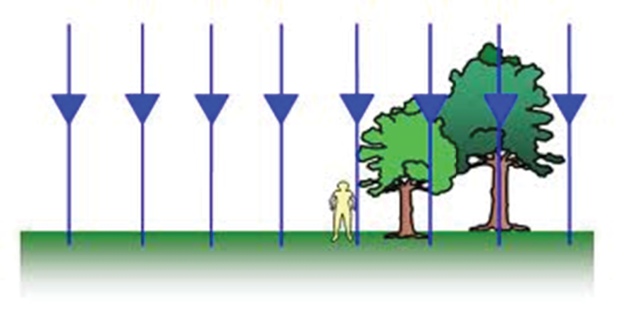
Figure 7. Earth’s Electric Field Lines of Force 22
V = approximately 40,0000 volts at ionoshere.2 Qearth2 = -3.2 x 10-13Coulomb/cm²= Positive Charge (at ionosphere as shown)
= Negative Charge (electrons in earth and tree as shown)

Electron Flow Diagram

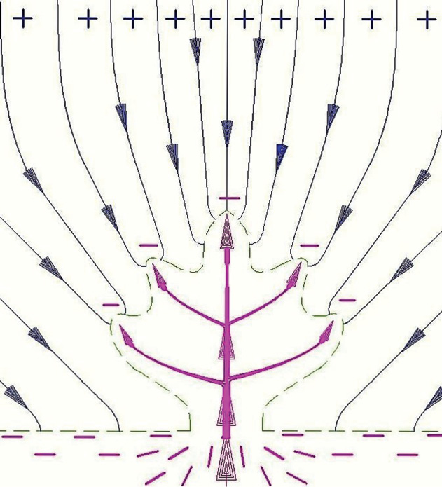
$C:\Users\Arde\Pictures\WJ pictures\Electric Field Lines of Force Diagram.jpg$

Figure 8. Electric Field Lines of Force and Electron Flow Diagram

The above Figure 8 drawing is based on Electron Flow Notation^23.

Figure 8 above is based on the voltage recordings of multiple trees and plants as shown in Appendix B-E. The recordings show the plants have the highest voltage in the stem or trunk. The voltage then drops progressively at the branches and branch tips. Therefore the electrons are entering the roots and traveling to the branch tips.

The electron density in the air ne within the Figure 8 green dashed line around the hypothetical 2 meter tree is calculated in Appendix J. n_e = 1.9 • 10¹⁶ electrons/m³

At the green dashed line in Figure 8, the electron density ne equals the ion density ni, (n_e = n_i) therefore the electron restoring force F_e = 0.

Infrared energy produces EZ water in the roots, trunk and branches and xylem transports protonated water to the branch tips. While Figure 8 only pictures electrons, see Figure 26 for both electrons and protons near the bud.

Electron Source Experiment

Faraday Cage Test Chamber:

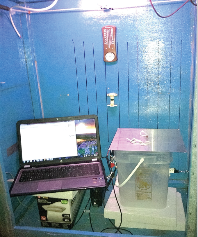
Picture 6. Electron source experiment- grounded Faraday cage test chamber above.

Above Faraday cage test chamber = 4’ x 3’ x 2’ used for running plant experiments with varied humidity and electric fields.

The Figure 9 and 10 graphs below show the electrons causing the negative stem voltage are coming from or through the water, entering the roots and flowing up to the stem when the sprout is rotated to touch water.

The Appendix E, Figure 21 Corn Leaf Recording – August 2013 shows a similar steady negative voltage on the leaf as seen above on the stem of these two corn sprout recordings.

The EZ zone of the water in the above test chamber has concentrated free moving electrons (page 79). ¹

Why are electrons flowing towards the buds? Protons inside the bud from EZ Water electrostatically attract electrons and at least partially cause the flow of electrons towards the branch tips. Protons in leaf tips3 caused by proton pumps inside the bud is also a possible reason, as are positive charges from the Earth’s Electric Field focused on each bud on the branch tips.

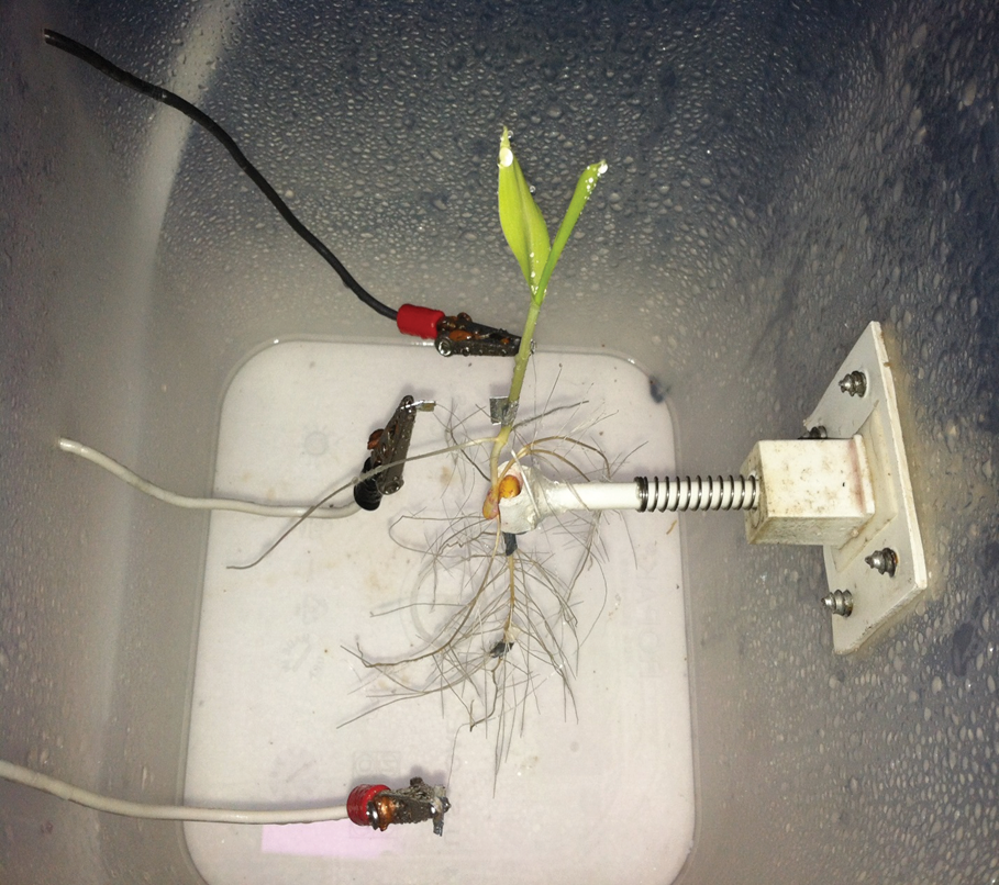
Picture 7. July 28, 2013 Corn Sprout growing without soil inside plastic tub. CH 1 POS lead to root. CH 2 POS lead to sprout stem. Common REF below seed. Fine aluminum wires were coiled and slid onto young sprout and root. Conductive tape placed around coil and gently squeezed, to ensure good bond between sprout and wire.

Figure 9. Young Corn plant in recording using PCSGU 250 oscilloscope

August 2013 Corn sprout Test inside Faraday Cage Graph 1&2 below

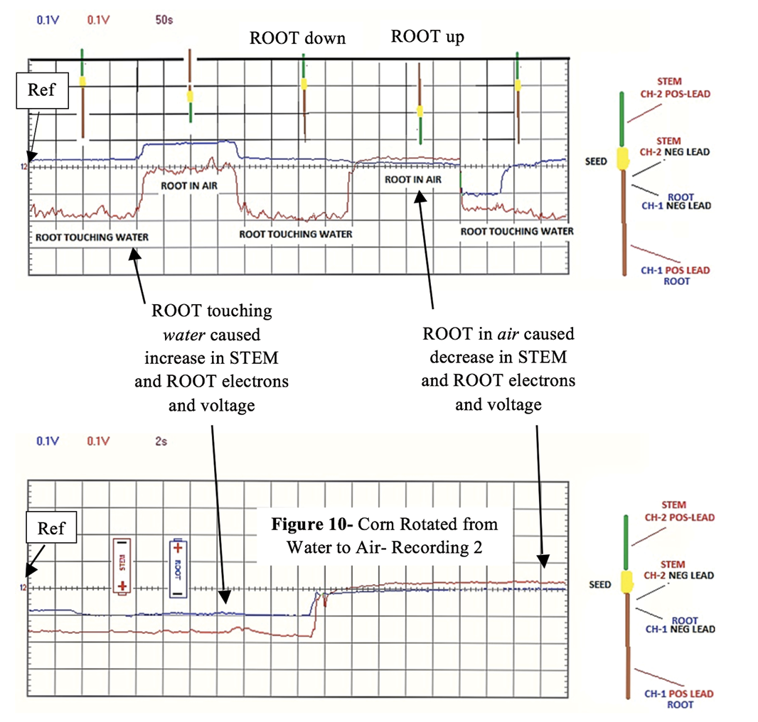
Figure 10. Young Corn plant inside Faraday Cage recording using PCSGU 250 oscilloscope
Vertical axis = Volts/division on both Figure 9 and Figure 10 recordings.
Figure 9 and 10 above CH 1 (Blue) = 0.1V/div. CH 2 (Red) = 0.1 V/div.
Horizontal axis = Time/division on all recordings. (Fig. 9 = 50 sec/div, Fig. 10 = 2 sec/div)

Horizontal Electric Field Corn Plant Experiment

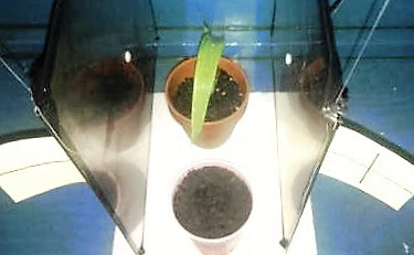
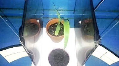
$C:\Users\Arde\Pictures\WJ pictures\7.28.2014 6.06 am cp.jpg$

Picture 8. 7-28-2014 6:06 am – Experiment start

7-28-2014 6:06 am Corn plant between suspended and isolated 12” sq. SS plates, 6” apart. Left plate = 0 VDC and Right plate = +60 VDC (electric field between plates approx. 2X earth electric field)

The stainless steel plates are a non-magnetizing type of SS.

The bottom of the SS plates are 6” above the faraday cage floor.

The front and rear SS plate edges are 6” away from the Faraday cage front and rear sides.

The backs of the SS plates are 15” away from the Faraday cage left and right sides.

Electrical tape was placed on plate edges and 6 mil plastic sheeting was added to the back of the plates to inhibit conductivity with the faraday cage.

The positive and negative voltage source leads are bonded at the center of each plate back with a small bolt. See the above bolt heads (white dots) at the center of the SS plates.

The voltage source was a continuous 60 VDC for the period of the experiment.

A continuous grow light is located inside and at the top of the Faraday cage. The temperature and humidity were ambient conditions for late July in Connecticut.

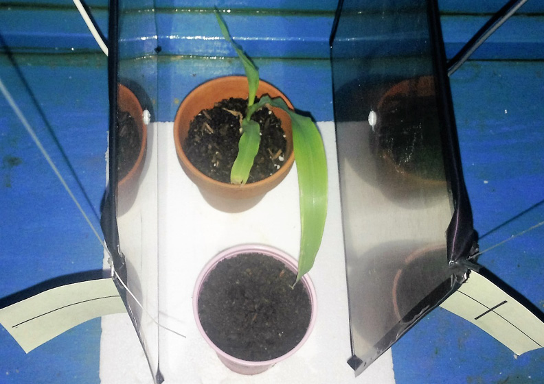
$C:\Users\Arde\Pictures\WJ pictures\7.29.2014 6.07 am cp.jpg$

Picture 9. 7-29-2014 6:07 am- 1 Day
7-29-2014 6:07 am – Corn plant has moved towards the positive plate after 24 hours.

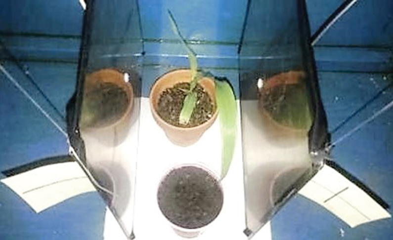
$C:\Users\Arde\Pictures\WJ pictures\7.29.2014 5.21 pm cp.JPG$

Picture 10. 7-29-2014 5:21 pm- 1.5 Days
7-29-2014 5:21 pm. More movement towards the positive plate.

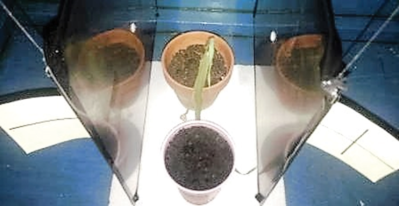
Picture 11. 7-31-2014 6:11 pm- 3.5 Days
7-31-2014 6:11am. Further movement towards positive plate.

Picture 12. 8-2-2014 8:50 am- 5.5 Days

Corn plant has collapsed and died. It is not known why the plant died, it possibly came in contact with the positive plate. The corn seed planted in the front cup failed to sprout.

Approximately 95% of this seed supply sprouted in previous tests.

This experiment is included in this paper to demonstrate the physical electrical effect on a plant from an artificial electric field. See Electricity in Agriculture and Horticulture by Prof. S. Lemstrom.⁴⁴ , Electroculture.

Conclusion

Part 1. Voltage Recording and Resistance Reading Methods and Procedure

With care, plant voltage recordings can be done using a digital voltmeter and PC-based oscilloscope.

Voltage recordings can be taken from 100’ away using coaxial cable to minimize ground induced noise.

PC based oscilloscope channels should be checked for independence.

Poor bonding results in bad data.

Resistance readings require a fresh multi-meter battery.

Resistance readings and red and black tape to mark the plugs was done to verify lead polarity.

Use ID tags on the branches.

To prevent interference, the recordings were done with the laptop on battery power, as well as lights and shop equipment shut off.

Conductive paste should be used with alligator clip voltage and resistance readings.

Part 2. Voltage Recordings

Negative voltage readings are caused by excess negative charges (electrons).

Plant voltage recordings for an Aspen tree, Spruce tree and Maple tree consistently showed the most electrons in the trunk, less in the branch, and the fewest electrons at the branch tips.

Figure 13, Aspen Recording shows decreasing voltage in the branch at dusk (8-9 pm, April 22, Zip code 49437). The decreasing sunlight caused a decrease in voltage at the branch base, but not the branch tip.

Billions of electrons are flowing towards the end of each branch tip/second.

In a tree’s space, hundreds of billions of electrons reach and leave the tree branch tips every second (Appendix I) and possibly forms an electron cloud in and above the tree with possible plasma properties, including frequency (Appendix K) and restoring force (Appendix J). ²⁴

The electrons attract the ions in the atmosphere that create Earth’s electric field and are very conductive. The electron cloud, because of its free electrons, is an excellent conductor, similar to plasma.

The relatively steady electrical flow in plants is possibly a small part of a larger circuit with the Earth’s electric field that obeys Kirchhoff’s second rule or loop theorem.15

Part 3. Electric Forces

The Resultant Electric Force at the branch tip is not strong enough to direct tip growth direction without the electron cloud restoring force. The electron cloud provides a repulsive restoring force F_e which nearly surrounds and pushes the bud’s slightly negative net charge towards the incoming earth’s electric field ions. See Figure 26.

The plant humidity field contributes an electric attractive force if the water droplets are polarized by the plants electric field. The water droplets are overall electrically neutral. Each water droplet will however become a dipole in the electric field. The dipoles align in the electric field and are able to transmit both a tensile force and compressive force because of their end to end electrostatic attraction to each other. See Appendix L – Tree Humidity Field.

Electrically directed growing branch tips create electric field lines of force branches.

The force calculations in Appendix M with an electron cloud show enough force to direct the tree and branch shape.

As possible evidence that the electron cloud exists within the tree volume, while doing GPS survey grade surveys I have noticed large trees interfere with the satellite signals to the GPS survey data collector. I also have noticed the satellite FM radio signal is lost as the car passes beneath large trees. See Appendix K – Electron Cloud Frequency.

The Appendix A, Figure 2, 1999 Electric Field Lines of Force Diagram display the same properties as tree branches.

Lichtenberg figures are a physical record of electrical flow.²⁶

Similar to Lichtenberg Figures, trees look like 3D solid copies of electric field “lines of force” and are physical records of electrical flow.

Once the bud becomes saturated with electrons, the measured electrons in Appendix B-E flowing continuously towards the branch tips are pushed into the air, these electrons possibly create an electron cloud around the plant which could be reacting with neighboring plant electron clouds. These electron clouds would repulse each other and the electrons in each cloud would repulse neighboring electrons. This electron cloud interaction would explain the observed plant to plant reaction repulsion.

The force calculations are meant for demonstration only and are not a full tree or multiple tree system model. Each branch has its own charges and electric field which interacts with all the tree branches and, earth’s electric field, and neighboring trees electric field and charges.

The source of the earth’s electric field (E) is assumed to be caused by more positive ions than electrons in the air. However, the earth’s surface here is shown with excess electrons which is generally accepted.

Part 4. Electron Source

Dipping a corn plant’s roots in water showed electrons from the water flowing into the roots, up to the stem, and causing a negative voltage. When the roots were removed from the water the root and stem electrons quickly decreased.

Separate experiments performed but not included in this paper show that dipping a moist dead tree branch in a plastic pail of water also showed electrons flowing up the branch. I believe this shows the effect of charge separation in EZ water. (Giving evidence to Dr. Gerald Pollack’s EZ water in his book The Fourth Phase of Water1).

Part 5. Electron Attraction to Plants

The voltage recordings in Appendix B-E show there are more electrons on the plant than in the soil at the ground rod. The recordings also show the electrons are moving towards the branch tips or buds. However, the electron flow direction in Electron Flow Notation²³ is from areas of high concentration to areas of low concentration, so the electrons should be flowing into the earth. Since the electron flow is opposite Electron Flow Notation, I believe, the earth’s positive electric field ions near the buds are attracting and concentrating earth electrons and EZ Water electrons towards the branch tips.

Part 6. Plant Reaction to Horizontal Electric Field

Applying a horizontal electric field of 10 volts/inch caused a corn plant to move towards the positive stainless steel plate before collapsing. Also a corn seed in a separate cup in the same field failed to sprout.

References

The Fourth Phase of Water, 2012 by Dr. Gerald Pollack, University of Washington

The Ascent of Sap in Tall Trees: a Possible Role for Electrical Forces. Johnson B. Independent Researcher, Oxford, UK https://waterjournal.org/volume-5/johnson-b#previous-measurements http://dx.doi.org/10.14294/WATER.2013.9

Leaf teeth, transpiration and the retrieval of apoplastic solutes in balsam poplar. T.P.Wilson, M.J. Canny, and M.E. McCully PHYSIOLOGIA PLANTARIUM 83: 225-232. Copenhagen 1991

Halliday and Resnick Physics Part I and II, 1966;

Chapter 26, Section 26-4, page 653 – Coulomb’s Law and permissibility constant є₀

Chapter 27, Section 27-2, page 665 – Electric field strength E

Chapter 31, Section 31-3, page 778 – Ohm’s law for metallic conductors

Chapter 26, Section 26-2, page 652 – Definition of amperage

Chapter 30, Section 30-2, page 746 – Parallel plate capacitor, cylindrical capacitor

Chapter 30, Section 30-2, page 747 – Cylindrical capacitor, capacitors in parallel

Chapter 30, Section 30-4, page 750 – Dielectric constant к

Chapter 39, Section 29-9, page 732 – Surface charge density by radius

Chapter 27, Section 27-4, page 670 – Coulomb force F, and electric field strength, E

Chapter 39, Section 29-9, page 731- Charge density on sharp points

Chapter 39, Section 29-9, page 733 – E near sharp points

Chapter 32, Section 32-3, page 793 – Kirchhoff’s Second Rule or loop theorem

Web References

Electrotropism:

https://en.wikipedia.org/wiki/Electrotropism

[3], polar growth with respect to an exogenous electric field

[4], directional signals in the repair and regeneration of wounded tissue

Appendix

Appendix A – Electric Field Lines of Force

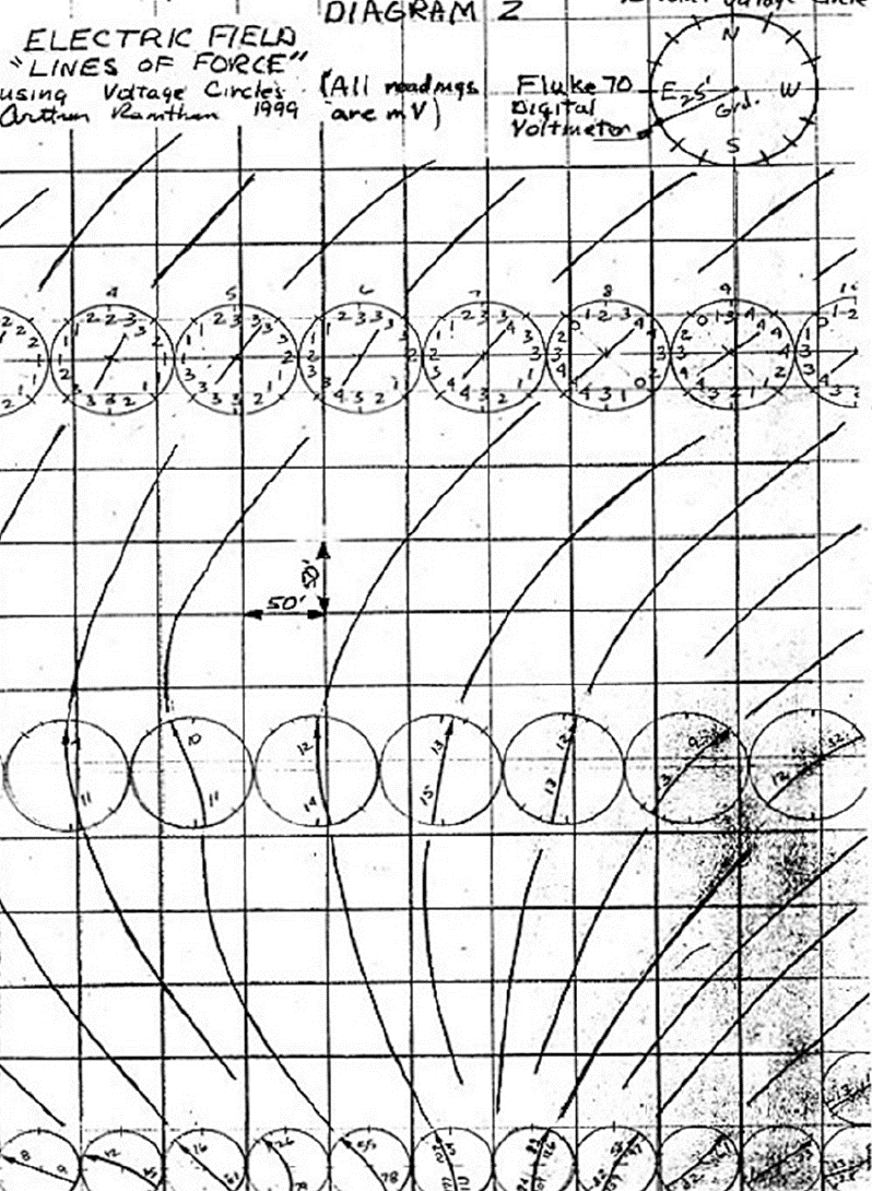
Figure 2. Electric Field Lines of Force developed using voltage circles.
The Diagram 2 drawing grid above is 50’ x 50’

Appendix B – Aspen Tree Voltage Recordings

$C:\Users\Arde\Pictures\WJ pictures\Aspen.jpg$
Picture 13. 80 foot Poplar tree voltage recording points

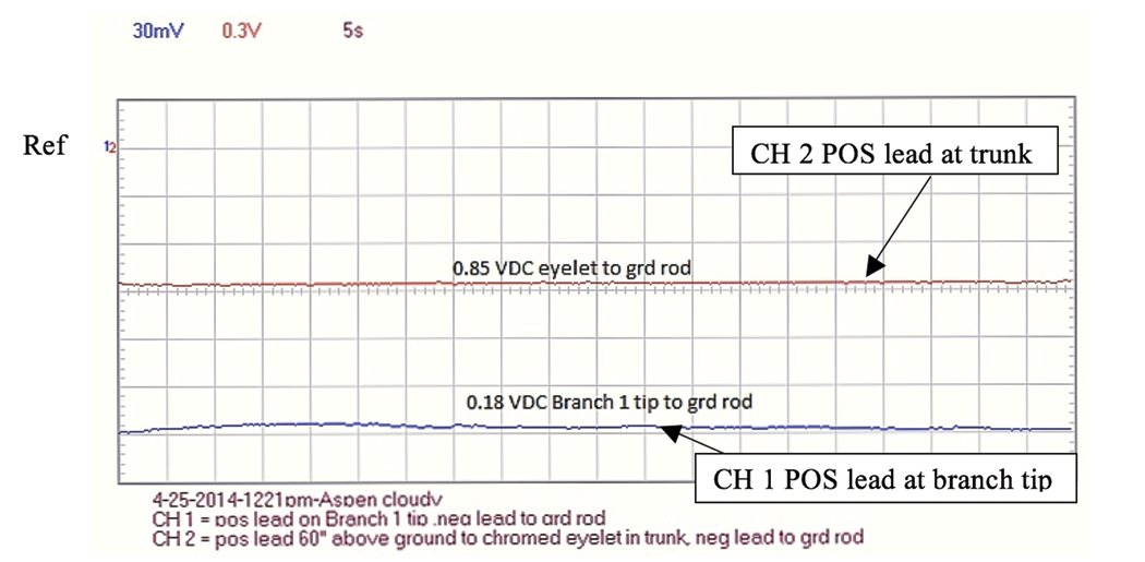
Figure 11. Aspen recording 1 using PCSGU 250 oscilloscope

Vertical axis = Volts/division on all recordings.

Above CH 1 (Blue) = 30mV/div. CH 2 (Red) = 0.3 V/div.

Horizontal axis = Time/division on all recordings. (Above Time/division = 5 seconds)

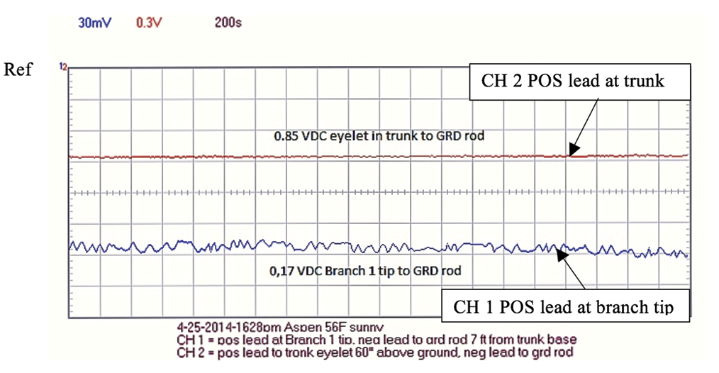
Figure 12. Aspen recording 2 using PCSGU 250 oscilloscope

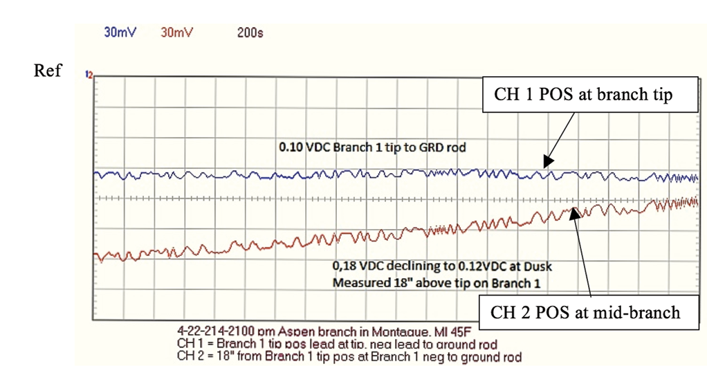
Figure 13. Aspen recording using PCSGU 250 oscilloscope.

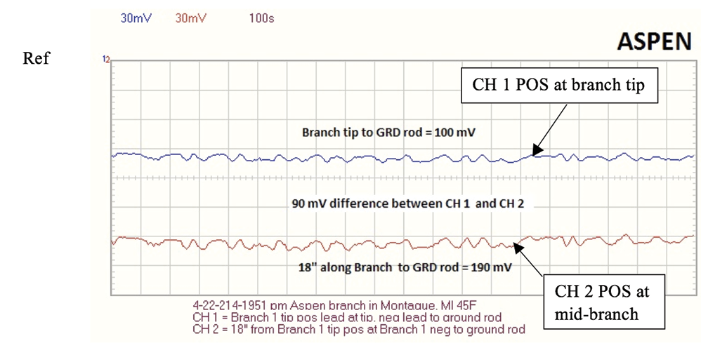
Figure 14. Aspen recording using PCSGU 250 oscilloscope. Note: Average ASPEN branch ohm readings = 2 Mohm from tip to 18” (7-13-14).

Appendix C – Blue Spruce Voltage Recordings

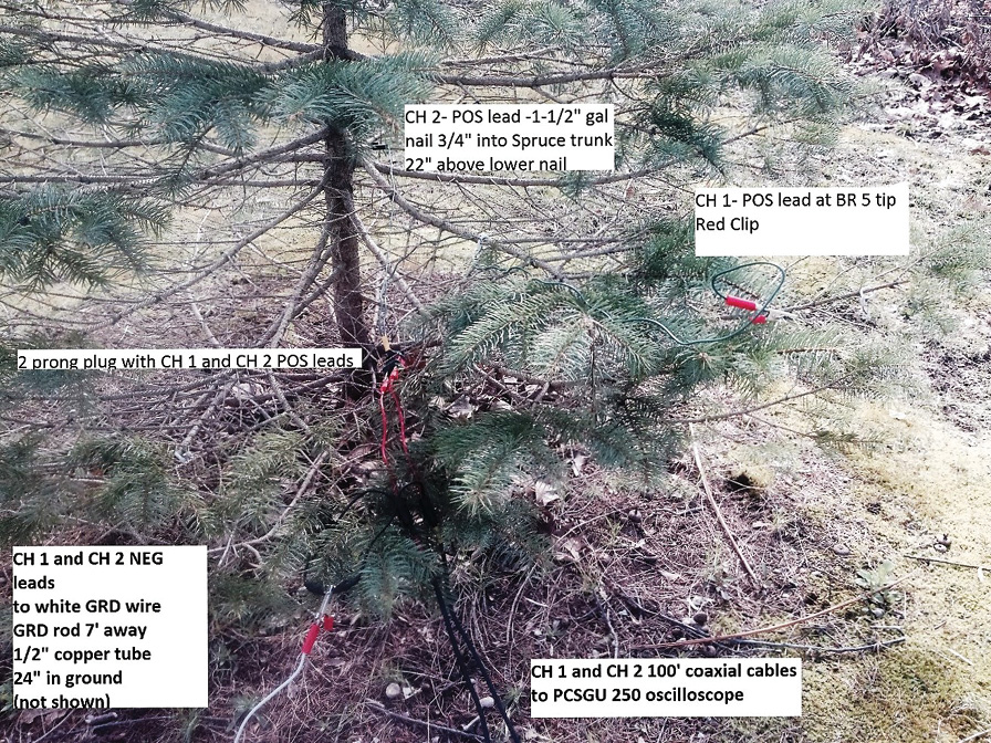
$C:\Users\Arde\Pictures\WJ pictures\Spruce pic.jpg$
Picture 14. 6 foot Blue Spruce voltage recording points.

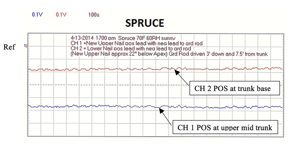
Figure 15. Blue Spruce recording using PCSGU 250 oscilloscope.

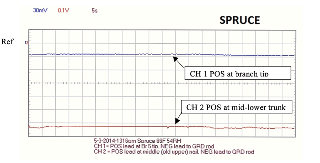
Figure 16. Blue Spruce recording using PCSGU 250 oscilloscope.

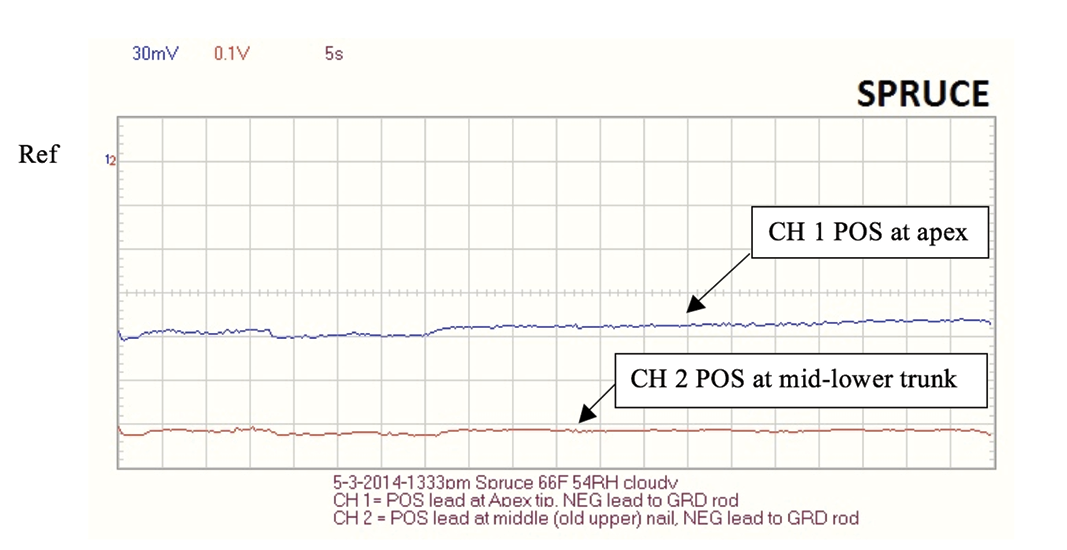
Figure 17. Blue Spruce recording using PCSGU 250 oscilloscope. Note: Spruce branch ohm readings were taken from tip to 18” and typically were 1-2 Mohm.

Appendix D – Maple Tree Voltage Recordings

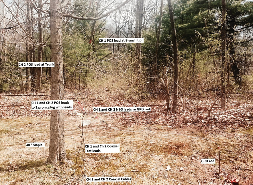
$C:\Users\Arde\Pictures\WJ pictures\Maple pic.jpg$
Picture 15. 40 foot Maple voltage recording points.

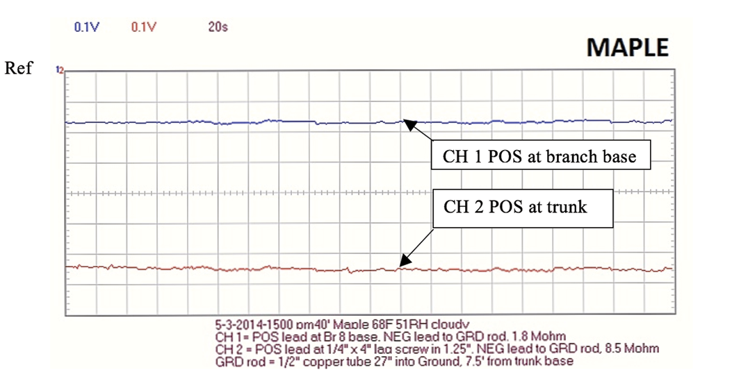
Figure 18. 40 foot Maple recording using PCSGU 250 oscilloscope.

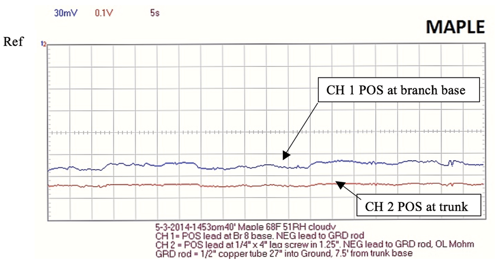
Figure 19. 40 foot Maple recording using PCSGU 250 oscilloscope.

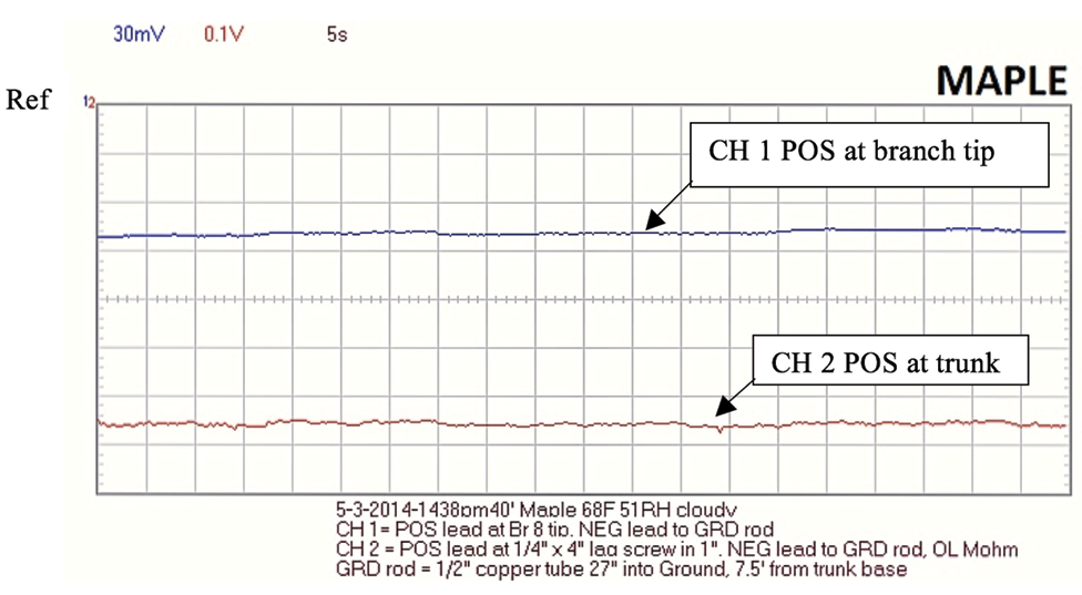
Figure 20. 40 foot Maple recording using PCSGU 250 oscilloscope. Note: Maple ohm readings October, 2014 from the trunk lag screw to GRD = 227 kOhm which indicates possible erroneous ohm readings above caused by weak Fluke 27 battery on earlier Maple ohm readings.

Appendix E – Small Corn in Clay Pot Voltage Recording

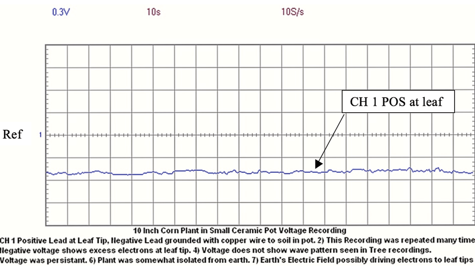
Figure 21. 8 inch Corn plant in clay pot recording using PCSGU 250 oscilloscope.

The recording above is of a small corn plant in a small clay pot. The recorded voltage on the corn leaf was a steady ^1/2 volt. This recording was repeated many times and shows excess electrons at the leaf tips. Shunting the voltage away on a different corn plant showed the voltage quickly returning after the shunt was removed.

Appendix F – Charge Inside Tip

Charge at Tip Using Plate Capacitors

Model tightly wrapped thin leaves in bud as capacitor plates in parallel.

C _{tip plate} = к є₀ A /d (Eq. 6)

Assume к = 78 (dielectric constant for water) ¹⁰

The measured total bud plate area (A) = 1.2 sq. in. = 7.7 cm² = 0.00077 m²

Assume: d (the distance between plates or leaf layers) = 0.01 mm or 1 • 10^-5 m

C _{tip plate} = к є₀ A /d = 78 • 8.9 •10^-12 • 0.00077 / 1 • 10^-5 = 5.4 •10^-8 farad

Equating Eq. 5 to Eq. 6, C =q/V = 5.4 •10^-8 farad

C _{tip plate} = V • 5.4 •10^-8 farad

V can be estimated from the V/m on the right side of Figure 4 below.

Assume E across tip = 1600 V/m and the average tip width b is 0.30 cm (0.003m)

V = 1600 V/m • 0.003 m = 4.8 volts

Q _{tip plate} = 4.8 • 5.4 •10^-8 farad = 2.6 •10^-7 coul (positive charge held by water inside tip)

Q _{tip plate} = 2.6 • 10^-7 coulomb (inside tip)

Appendix G – Charge Inside Trunk

A way to calculate trunk capacitance is to treat the water conveying vessels in the sapwood as pairs of parallel conductors. ³⁶

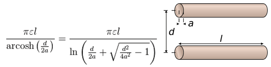
Figure 8 shows a vessel diameter as 7 μm (a = 3.5 μm)

Assume: a = 3.5 μm, d = 10 μm, l = 2 m, к= 78 for a capacitor with water as the dielectric.

C vessel pair = 78 • π • 8.9 • 10^-12 • 2 /ln (10/7 + (100/49 -1)^1/2) = 4.9 • 10^-9 farad/vessel pair

Assume 3 tree rings with average diameters = 50 mm, 40 mm, and 30 mm. The corresponding circumferences = 157 mm, 125 mm, and 94 mm.

Assume the Angiosperm diagram (Figure 23) below is 5 mm x 2.5 mm and contains 3 pair (6 total vessels).

Adding the ring circumferences together = 157+125+94 = 376 mm

Dividing 376 mm / 2.5 mm = 150 (2.5 mm sections each containing 3 vessel pairs)

Multiplying 3 vessel pairs x 150 sections = 450 vessel pairs

C trunk = 4.9 • 10^-9 farad/vessel pair • 450 vessel pairs = 2.2 x 10^-6 farad

Calculating the trunk charge:

C = q/V (Eq. 5)

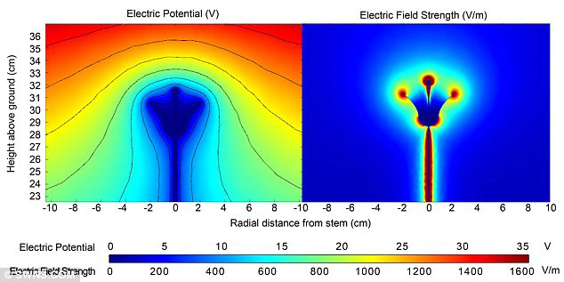
Figure 4. University of Bristol’s School of Biological Sciences, Plant Voltage Diagram (2013 Bee Research). ²⁵

Assume E = 1500 V/m (Figure 4 diagram on the right)

Assume the 1500 V/m is acting across the trunk width (b • 2) = 0.03 • 2 = 0.06 m

Therefore V = 1500 V/m • 0.06 m = 90 volts across the trunk

Q_trunk = V • C = 90 • 2.2 • 10^-6 = 2.0 • 10^-4 coulomb

Q_trunk = -2.0 • 10^-4 coulomb (inside trunk) (negative because trunk is losing EZ water protons in water transport to branch tips).

Early and Late Wood in Tree Rings

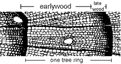
transverse view of a conifer tree ring
Figure 22. Conifer Tree Ring Diagram³³Earlywood 1. appears light in color, 2. cells have thin walls, large diameter.
Latewood 1. appears dark in color, 2. cells have thick walls, small diameter.

transverse view of an angiosperm tree ring
(transverse or cross-sectional view)
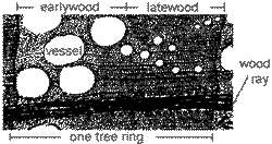
Figure 23. Angiosperm Tree Ring³³
Earlywood – cells have large diameter vessels
Latewood – cells: small diameter vessels

The above tree ring picture and vessel diagram reveal why tree rings can be considered capacitive conductors acting in parallel. The early wood has large open cells which holds and transports more water than the darker small diameter late wood cells.

Appendix H – Calculating the Electric Field Outside of the Branch Tip

“The electric field strength E at points immediately above a charged surface is proportional to the charge density σ so that E may reach very high values near sharp points” ¹³

For a spherical object, the surface charge density σ = q/4πR²

Where q = charge and R = radius of sphere

The measured length of the Laurel terminal bud is 1.45 cm and the width is .64 cm.

Average R = (1.45 + .64)/4 = 0.52 cm

Treating the bud as a sphere, the surface area A _bud = 4π 0.52² = 3.43 cm²

Assume the sharp tip R is 0.3 cm and a hemisphere.

A _point = 2 πR² = 0.57 cm²

The Appendix H calculated internal positive charge at the tip is 2.6 • 10^-7 coulomb.

If -2.6 • 10^-7 coulomb of electrons are outside the tip, the overall net tip charge is zero.

However, the earth’s electric field will pull more electrons to the top of the tip so the electrons will be offset and a net negative charge will result.

Net charge: Assume 2% extra of -2.6 • 10^-7 coulomb is offset at the tip = -5.2 • 10^-9 coulomb

Q _{tip net} = -5.2 • 10^-9 coulomb

The charge density ratio is A _bud / A _point = 3.43 / .57 = 6 (increases E field by factor of 6)

E = (1/4πє₀) q/R² (Eq. 2) where r is radial distance from the charge q outside the tip.

Assume r = 0.01 m (1 cm)

E = 6 • 9 • 10⁹ • -5.2 • 10^-9/ .01² = -2,808,000 V/m

If the electrons are pulled 10 cm away from the bud tip then E = -28,080 V/m.

(Coronal discharge³⁷ occurs at approximately 3,000,000 V/m)

So a small charge can create a large local electric field.

“If the charged conductor has sharp points, the value of E in the air near the points can be very high.” ¹⁴

Blue spruce needles are very sharp, so a very small charge at the tip of each needle creates an intense electric field which is attracted to and pulls in the earth’s electric field ions.

This E field around the bud seems unreasonably high. However if an electron cloud is around the bud the E field is decreased. The permittivity constant є₀ is for free space or air and does not model the electrons around the bud or between the bud and trunk in my opinion.

Appendix I – Bud Electron Cloud Field

Assume each branch tip for the hypothetical 2 meter tall tree is receiving 25% of the Aspen tip amperage calculation on page 12 above or 70,000,000,000 electrons/second.

From Appendix H, Q _{tip electrons} = -2.6 • 10^-7 coulomb

Q _{tip net} = -5.2 • 10^-9 coulomb (assuming 2% more electrons than bud ions)

Q _{tip total electron} = Q _{tip electrons} + Q _{tip net} = (-2.6 • 10^-7) + (-5.2 • 10^-9)

Q _{tip total electron} = -2.65 • 10^-7 coulomb (electrons around bud which are held by bud ions and Earth’s Electric field ions)

The 70 billion electrons/second moving towards the bud are moving at an unknown speed and are likely pushed off the branch and into the air by the static electron charge Q _{tip total electron} near the bud.

Electron # = -2.65 • 10^-7 coulomb / 1.60 x 10 ^-19 coulomb/electron = 1.65 • 10¹² electrons/bud

If the static electrons forms a 1 cm radius sphere of volume = 4.2 cm³, then the static electrons density near the bud is 3.9 • 10¹¹ electrons/cm³ = 3.9 • 10¹⁷ electrons/m³.

The measured length of the Laurel bud in Appendix H = 1.45 cm

Appendix J – Tree Electron Cloud Field Restoring Force

Electron Cloud as Plasma Calculation

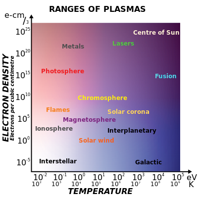
Figure 24. Plasma Scales ³⁹

See ³⁸ 1.1.2 Plasmas are Quasi-Neutral

If a gas of electrons and ions (singly charged) has unequal numbers, there will be a net charge density, ρ. ρ = n_e (−e) + n_i (+e) = e (n_i − n_e) n_e = electron density, n_i = ion density.

E = є₀ • x / є₀ (assume x = distance from the center to the edge of plasma field)

“This results in a force on the charges tending to expel whichever species is in excess. That is, if n_i > n_e, the E field causes n_i to decrease, n_e to increase tending to reduce the charge.” ³⁸

However, in the case of the electrons flowing off the tree branches and tips, the resulting electron cloud will have more electrons than ions.

Therefore n_e > n_i, the E field causes n_e to decrease, n_v to increase tending to reduce the charge from electrons.

Assume there is a 1% more electrons than ions. ∆n = (ne – ni)

Therefore: ρ = ∆n e and F_e = ρ • E (Eq. 2 per unit volume)

Assume: ∆n / n_e = 1%, x = 0.5 m. (assume x = distance from center of plasma field to edge of plasma field)

F_e = restoring force per unit tree volume from electrons at distance x is.

F_e = ρ • E = ρ ² x / є₀ = (Δn • e)² • x / є₀ F_e is a radiating force. (nt/m³)

Solve for Δn;

(Δn • e)2 = F_e • є₀ / x

Δn = (F_e • є₀ / x) ^1/2 / e (electrons/m³)

Assume F_e = 50 nt/m³

Δn = (50 • 8.9 • 10^-12/0.5) ^1/2/ 1.6 • 10^-19 = 1.9 • 10¹⁴ electrons/m³

∆n = (n_e – n_i)

n_i = 0.99 n_e

∆n = (n_e – 0.99 n_e)

∆n = n_e (1-0.99)

n_e = 1.9 • 10¹⁴ / 0.01

n_e = 1.9 • 10¹⁶ electrons/m³

Assume the Tree Electron cloud field boundary is the dashed line around the Figure 8 tree and the tree is the hypothetical 2 meter tree.

From Appendix I, there are 70 billion electrons/second/bud flowing towards each bud.

Assume this tree has 20 branches and 80 branch tips and each push an equal amount of electrons to the air/second.

100 branches and buds • 7 • 10¹⁰electrons/second = 7 • 10¹²electrons/second

Assume a conical tree volume = πR² • h/3 = π • 2/3 = 2 m³ (r = 1 m and h = 2 m)

Quasi neutral plasma #e = ∆n electrons/m³ • 2 m³ = 3.8 • 10¹⁴ electrons

3.8 • 10¹⁴ electrons/ 7 • 10¹² electrons/second = 1 minute (1% electron refresh time)

Electron density, n_e = 1.9 • 10¹⁶ electrons/m³ = 1.9 • 10¹⁰ electrons/cm³

Similar electron density to the chromosphere in Figure 24 above.

F_e is the Coulomb repulsive force within the tree electron cloud field. The tree electron cloud field reduces the voltage and electric field within the 2m³ tree volume.

If the earth’s electric field (E_F) outside of the tree is quasi-neutral, then it contains almost as many electrons as positive ions. If the electrons around the bud attract the positive ions in E_F, the E_F electrons will concentrate between the buds and form a barrier or electron canopy to contain the tree electron cloud. See 6 in Figure 25 below.

The electron charge density ρ and electron restoring force will increase with height up the tree. This fits with the observation that branches at the top of the tree show stronger electric field lines of force than branches near the bottom of the tree.

Why would electrons stay near the tree? Looking at the Electric Field Lines of Force Diagram Figure 1 in Appendix A you notice the electric field lines of force are bending. These electrons are bending around another electric field which is blocking their way. Also, these electrons in Figure 1 are trying to “complete the circuit” and get back to the substation transformer.

In the tree trunk, the EZ Water separates protons and electrons and is acting as a transformer. The protons flow towards the branch tips in the xylem. It seems the electrons don’t want to leave the protons behind as they follow along on the branches. Even after the electrons are forced into the air within the tree volume they won’t want to leave. The electrons need to get back to the protons is what causes them to build up and create an electron cloud with a restoring force in my opinion.

Appendix K: Plasma Frequency ⁴¹

An expression for the dielectric constant of a plasma is є = 1 – ωP2/ω2

Where: ω_P = plasma frequency, ω = incident radiation frequency

ω_P = [n_e • e²/є₀ • me]^1/2 n_e = 1.9 • 10¹⁶ electrons/m³ (Appendix J)

ω_P = [1.9 • 10¹⁶ • (1.6 • 10^-19)² / 8.9 • 10^-12 • 9.11 • 10^-31]^1/2

ω_P = 7.7 • 10⁹ / sec

Therefore, if the incident radiation is a GPS signal at 1GHZ, the signal will be reflected by the tree.

Therefore, if the incident radiation is an FM radio signal at 100 MHZ, the signal will be reflected by the tree. See discussion. ⁴²

While doing GPS survey grade surveys I have noticed large trees interfere with the satellite signals.

I also have noticed the satellite FM radio signal is lost as the car passes beneath large trees.

Signals with smaller frequency than ω_P will be interfered with by the plasma. ⁴¹

Appendix L – Tree Humidity Field

Plants need humidity and create humidity to stay healthy. ⁴⁰

Humidity water droplets given off by the tree have a net charge of zero.

However, these water droplets exposed to an electric field will be polarized and become a dipole.

The cloud of polarized droplets will be electrostatically connected in three dimensions.

The electrostatic connections are able to transfer small push and pull forces within the humidity cloud.

Humidity droplets polarized by the tree and earth electric field could have a similar effect on the bud as an electron cloud.

Picture 16 shows corn roots growing towards the bottom left corner of the test chamber. There is a humidifier below the white foam sheet in the picture. The foam sheet is forcing the humidity water droplets towards the chamber corners. The humidity field extents from the corners upwards and towards the middle and the roots. I believe the earth’s electric field is polarizing the humidity. The roots are then electrostatically attracted to the polarized water droplet field. So the roots are being electrostatically attracted to the humidity in my opinion.

Sept_Oct 2011 123

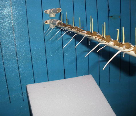
Picture 16. Hydrotropism- Roots Attracted to Humidity ⁴²

Appendix M: Calculation of Forces at Branch Tip for below FBD 2 (with electron cloud)

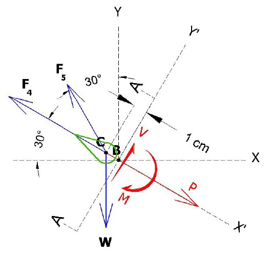
Figure 25. Vector Force Free Body Diagram 2– (FBD 2) (not to scale)

Figure 26. Bud Local Charge System (Not to scale).

In Figure 26 below left, the numbers 1-9 mean:

1. Q _{tip plate} = 2.6 • 10^-7 coulomb (protons inside tip) See Appendix F

2- Q _{tip net} = -5.2 • 10^-9 coulomb (2% of electrons outside tip) See Appendix H

3. Boundary of tip electrons, Q _{tip total electron} = -2.65 • 10^-7 coulomb, Appendix I

4. Force boundary between the tip electron cloud restoring force field and the tree electron cloud restoring force F_e. The tip electron cloud restoring force = the tree electron cloud restoring force. See Appendix J

5. “Hole” in the tip electron cloud caused by concentrated earth electric field ions neutralizing the concentrated electrons.

6. Concentrated earth electric field ions drawn in by Q _{tip total electron}.

7. Tree electron cloud field. See Appendix J

8. Earth Electric Field

9. the boundary between tree and earth electric fields. At this boundary, the number of electrons = the number of ions, therefore F_e = 0. The green dashed line in Figure 8 – Electron Flow Diagram also represents the “9” boundary.

In Figure 5 above only F₄, F₅, and W are the forces involved. The calculation using the electron cloud restoring force, F_e, replaces the charge to charge forces (F₁, F₂, F₃) shown in Appendix O –Figure 5 because F_e is a radiating force surrounding most of the bud.

The electron cloud restoring force F_e boundary is shown by 4 in Figure 26 above.

Calculating F₄

Assume the tree electron cloud and bud electron cloud has no effect on internal bud charge so use є₀ and the bud capacitance calculation already used the dielectric constant к = 78, because of the water in the bud plates acting as a dielectric. See Appendix F.

Q_{tip internal} repels Q_cm (internal charge 1 cm from tip)

F₄= internal force at branch tip caused by like charge repulsion.

F = (1/4 πє₀) q₁ • q₂ / R² Coulombs Law (Eq. 2)

Q _{tip plate} = 2.6 • 10^-7 coulomb (Appendix F) (inside tip)

Assume; Qcm = Q _{tip plate} /2 = 1.3 • 10^-7 coul, r = 0.01 m (1 cm), θ = 30^o

F₄= 9 • 10⁹ (2.6 • 10^-7 • 1.3 • 10^-7) / .01² = 3.0 nt

F₄ = 3.0 nt

(Pushing 30^o from horizontal upwards and to left on the tip in the FBD) (Like charges repel)

Calculating F₅

Q_TIP electron cloud is repulsed by Tree electron cloud restoring force,

See Figure 26 above.

It is logical to assume all the electrons creating negative voltage and shown in Figures 11-21 in Appendix’s B-E which are flowing towards the branch tips create a negative electron cloud around the bud.

Assume the bud electron cloud attracts equal numbers of the earth’s electric field ions. These electrons and ions cancel each other.

This creates a low pressure “hole” in the electron cloud. See Figure 26, label 5.

The tree electron cloud restoring force F_e then pushes or buoys the tip towards the hole in the negative bud electron cloud.

From Appendix J, F_e = 50 nt/m³ (an assumed force used to calculate electron cloud charge density).

Assume half the negative bud electron cloud opposite the “hole” is repulsed by the tree electron cloud, and this hemisphere has a 0.15 meter radius.

The volume of a hemisphere with 0.15 m radius = 4/3πr³/2 = 0.007 m³

Use the hemisphere volume multiplied by F_e to approximate F₅.

F₅ = 50 nt/m³ x 0.007 m³ = 0.35 nt

F₅ = 0.35 nt

Pushing 60o from horizontal upwards and to left on the tip in the FBD 1.

Calculating W

W = mg, m = 0.14 gram (average of 8 Laurel buds), g = 9.8 m/sec²

W = 0.00014 • 9.8 = 0.0014 nt

W = 0.0014 nt (gravity acting vertically down in the FBD 1)

Branch tip force summary;

F₄ = 3.0 nt pushing 30^o up and to the left on the branch tip in FBD 1)

F₅ = 0.35 nt (pulling 60o up and to the left on the branch tip in FBD 1)

W = 0.0014 nt (acting down on the branch tip in FBD 1)

Appendix N Determining reactions P, V, M, R, θ in FBD 2 (with electron cloud)

(cos 30^o = 0.866, cos 60^o = 0.5)

∑ Forces = 0

P – F₄ – 0.866 F₅ + 0.5 W = 0

P = (3.0 + 0.30 – 0.0007) nt

P = 3.3 nt (acting along X’)

∑ Forces = 0

V + 0.5 F₅ – 0.866 W = 0

V = (- 0.175 + 0.0012) nt = 0

V = -0.17 nt (acting along Y’)

∑ M_B = 0

M + 0.5 F₅ – 0.866 W • (1 cm) = 0

M = (-0.175 + 0.0012) nt-cm = 0

M = -0.17 nt-cm (rotating around B)

Assuming equal and opposite forces in FBD 3 below:

F_X^’ = (-P) = -3.3 nt

F_Y^’ = (-V) = 0.17 nt

Finding the resultant force (R) and angle θ:

R = (F_X^’2+ F_Y^’2) ^1/2 = (-3.3² + (0.17²))^1/2 = 3.3 nt

R angle θ = arctan (y/x) = arctan (0.17/3.3) = 3 degrees above X’

R = 3.3 nt @ 33^o

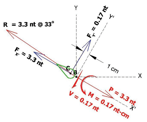
Figure 27. Resultant Force FBD 2 with Electron cloud

Appendix O Calculation of Forces at Branch Tip for below FBD 2 (no electron cloud)

Calculations Assumption Summary

For F₁,

It is assumed Q_{tip net} = -5.2 •10^-9 coul r = 0.5 meter

Q_EARTH = (-3.2 • 10^-13 coul/cm²) • (100 cm)²/m² = -3.2 • 10^-9 coul/m²

For F2

It is assumed Q_{tip net} = -5.2 •10^-9 coul , Q_trunk = -2.0 • 10^-4 coul, r = 1 meter

For F3

It is assumed Q_{tip net} = -5.2 •10^-9 coul, Q_BRANCH= 7 • Q_{tip net} = -3.6 •10^-8 coul, r = 0.2 meter, θ = 45^o (In Q_BRANCH= 7 • Q_{tip net}, the number 7 is an assumed factor based on the branch being much bigger and holding more charge than the branch tip)

For F₄

It is assumed Q_{tip net} = -5.2 •10^-9 coul , Q_25mm = Q_{tip net} /2 = -2.6 • 10^-9 coul,

r = 0.025 meter, (25 mm), θ = 30^o above horizontal

Note: The assumption such as 25 mm between the internal charges creating F₄ could easily be 1 mm or 1 μm.

For F₅

It is assumed E_BRANCH = -1600 V/m (See above Figure 4– Electric Field at branch tip)

θ = 30^o above horizontal, Q_{tip net} = -5.2 •10^-9 coul

For W

It is assumed, mass of sectioned tip = .00014 kg (0.14 gram)

Electric and Gravity Vector Force Diagrams

Free Body Diagrams at Branch Tip

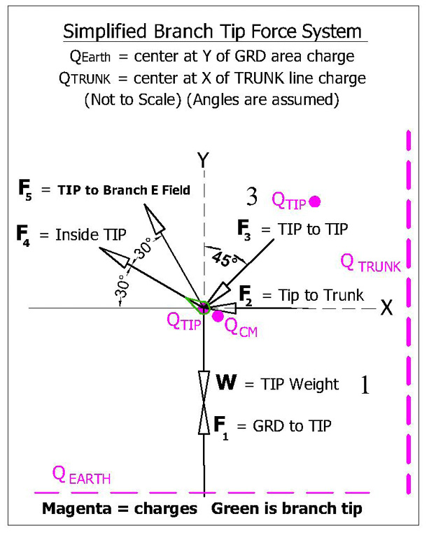
Figure 4. Vector Force Free Body Diagram 1– (FBD 1) (not to scale)

2D (FBD 1) branch tip vector forces are for demonstration calculations.

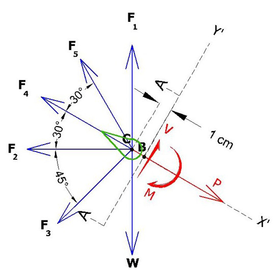
Figure 5. Vector Force Free Body Diagram 2– (FBD 2) (not to scale).

In FBD 2, the Branch tip is sectioned at A-A using the “Method of Sections.” V = shear force, M = bending moment about B, and P = axial force. V, P, and M bring the sectioned tip into static equilibrium. Coordinate axis is rotated 30^o to match A-A.

Calculating F₁:

Q_tip interacts with E_earth (earth electric field created by σ)

Substituting and rearranging Eq.2 (E = F /q0) F1= Q_tip • E (Eq. 2)

Where E = σ/2є₀ σ = -3.2 • 10^-9 coul/m² (Figure 7, Earth’s Electric Field Diagram above)

E = -3.2 • 10^-9 / 2 • 8.85418 x 10^-12 = 180 V/m

Q_{tip net} = -5.2 • 10^-9 coul

Assume the distance between the earth and the tip is r = 0.5 m

E at 0.5 meter = 90 V/m

F1 = (-5.2 • 10^-9 coul • -90 V/m) = 4.7 • 10^-7 nt

F1 = 4.7 • 10^-7 nt

Calculating F2:

Q_{tip net} interacts with Q_trunk (charge in trunk) (tip to trunk force)

F = (1/4 πє₀) q₁ • q₂ / R² Coulombs Law (Eq. 2)

Assume; Q_{tip net} = -5.2 • 10^-9 coul, Q_trunk = -2 • 10^-4 coul, r = 1 meter

F₂= 9 • 10⁹ (-5.2 • 10^-9 • -2 • 10^-4) / 1² = 0.01 nt

F₂ = 0.01 nt (pushing horizontally left on the branch tip in the FBD) (like charges repel)

Calculating F3:

Q_{tip net} interacts with Q_branch (adjacent branch charge) (tip to branch above)

F = (1/4 πє₀) q1 • q2 / R² Coulombs Law (Eq. 2)

Assume; Q_{tip net} = -5.2 • 10 -9 coul, QBRANCH = 100 • Q_{tip net} = -5.2 • 10^-7 coul, r = 0.2 meter,
θ = 45^o

F3= 9 • 10⁹ (-5.2 • 10^-9 • -5.2 • 10^-7) / .2² = 0.0006 nt

F3 = 0.0006 nt

Calculating F₄:

Q_tip _plate repels Q_cm (internal charge 1 cm from tip)

F₄= internal force at branch tip caused by like charge repulsion.

F = (1/4 πє₀) q₁ • q₂ / R² Coulombs Law (Eq. 2)

Q _{tip plate} = 2.6 • 10^-7 coulomb (Appendix F) (inside tip)

Q_cm = Q _{tip plate} /2 = 1.3 • 10^-7 coul, r = 0.01 m (1 cm), θ = 30^o

F₄= 9 • 10⁹ (2.6 • 10^-7 • 1.3 • 10^-7) / .01² = 3.0 nt

F₄ = 3.0 nt

(Pushing 30^o from horizontal upwards and to left on the tip in the FBD) (Like charges repel)

Calculating F₅
Q_TIP interacts with E_earth (earth electric field immediately above tip)

Substituting and rearranging Eq.1 (E = F /q₀) F₅ = Q_tip • E_{tip air} (Eq. 1)

E _{tip air} = 2,484,000 V/m (Appendix H)

θ = 60^o

Q _{tip net} = -5.2 • 10^-9 coul (Appendix H)

F₅ = -E • q₀ = -2,808,000 • -5.2 • 10^-9 = 0.015 nt

F₅ = 0.015 nt

(Pulling 60^o from horizontal upwards and to the left on the branch tip in the FBD)

Calculating W

W = mg, m = 0.14 gram (average of 8 Laurel buds)(0.00014 kg) and g = 9.8 m/sec²

W = 0.00014 • 9.8 = 0.0014 nt

W = 0.0014 nt (gravity acting vertically down in the FBD 1)

Branch tip force summary;

F₁ = 0.00000047 nt (pushing vertically up on the branch tip in FBD 1)

F₂ = 0.01 n (pushing horizontally left on the branch tip in FBD 1)

F₃ = 0.0006 nt (pushing 45^o down and to the left on the branch tip in FBD 1)

F₄ = 3.0 nt (pushing 30^o up and to the left on the branch tip in FBD 1)

F₅ = 0.015 nt (pulling 60o up and to the left on the branch tip in FBD 1)

W = 0.0014 nt (acting down on the branch tip in FBD 1)

Appendix P:Determining Reactions P, V, M, R, θ in FBD 2 (No Electron Cloud)

(cos 15^o = 0.966, cos 30^o = 0.866, cos 60o = 0.5, cos 45o = 0.707, cos 75^o = 0.259)

∑ Forces = 0

P – 0.5 F1 – 0.866 F2 – 0.259 F3 – F₄ – 0.866 F₅ + 0.5 W = 0

P = (+ 0.00000023 + 0.0087 + 0.00016 + 3.0 + 0.013 – 0.0007) nt

P = 3.0 nt (acting along X’)

∑ Forces = 0

V + 0.866 F1 – 0.5 F2 – 0.966 F3 + 0.5 F₅ – 0.866 W = 0

V = (-0.000004 + 0.005 + 0.00058 – 0.0075 + 0.0012) nt = 0

V = -0.0007 nt (acting along Y’)

∑ M_B = 0

M + 0.866 F1 – 0.5 F2 – 0.966 F3 + 0.5 F₅ – 0.866 W • (1 cm) = 0

M = (-0.000004 + 0.005 + 0.00058 – 0.0075 + 0.0012) nt-cm = 0

M = -0.0007 nt-cm (rotating around B)

Assuming equal and opposite forces in FBD 3 below:

F_X^’ = (-P) = 3.0 nt

F_Y^’ = (-V) = 0.0007 nt

Finding the resultant force (R) and angle θ:

R = (F_X^’2+ F_Y^’2) ^1/2 = (3.02 + (0.00072))^1/2 = 3.0 nt

R angle θ = arctan (y/x) = arctan (0.0007/3.0) = 0.013 degrees above X’

R = 3.0 NT @ 30.01o

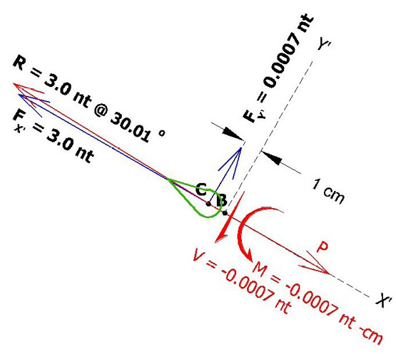
Figure 6. Vector Force Free Body Diagram 3– (FBD 3) (not to scale).

Calculated forces in Appendix O and P in FBD 1 and FBD 2 are reduced to above forces and moment in FBD 3.

Discussion with Reviewers

Reviewer No. 1

Q1: In one experiment it is shown that placing a maize plant root in water induces a negative voltage reading at the root tip. The conclusion is that this is mediated by EZ water. However, another possibility is that charged ions species in the water acted as the charge carriers. If this experiment were repeated with deionized (DI) water, would the same effect be observed?

This would be a good experiment to run. The DI would become corrosive (acidic) when exposed to air. When the EZ layers form, the H to O ratio changes from 2:1 to 3:2. the hexagon pushes out the extra H+ and the EZ becomes negative. The extra H+ in the DI would attack the EZ, but because the EZ pushes out H+ normally, I suspect the EZ would survive and the pH in the water outside the EZ would be even lower than normal water.

Q2: Dead wood is a known insulator, not a conductor. In addition, resistance is inversely proportional to electrical conductance, and the resistance values reported here are very high (on the order of Mega Ohms). In light of this, is it probable that woody plant tissue conducts electrons?

I believe the moisture in the wood is the primary conductor. When I took resistance readings of live branches, the current induced by the voltmeter seemed to be polarizing the water in the branch because the resistance slowly decreased before stabilizing. An earlier experiment I ran showed a 40 fold decrease in resistance between two copper tubes in a pan of water when a 12 volt 10 amp current was applied.

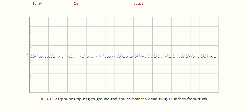
Voltage readings on a small dead spruce branch showed only a couple mV. See below 10-3-13 graph.

Q3: Woody plants are known to transport water and electrically-charged ions and auxin hormones. In an experiment that was similar to the root in the water experiment reported here, it was shown that putting auxin and auxin transport inhibitors into the water inhibited the electrotropic response, suggesting that electropism may be mediated by auxins.1 It has also been shown that the electrotropic response in Camellia pollen tubes is mediated by calcium ion concentrations.2 It has also been suggested that similar voltage readings in charophyte may be caused by the flux of acidic and basic ions, although this is controversial.3 4 Even pure water can conduct acidic positively-charged protons by the Grotthuss mechanism. With this in mind, might the transport of electrically-charged protons, ions, and auxin hormones be sufficient to account for the observed voltages and calculated currents?

Yes. The EZ water produces protons as shown in Figures 7 and 8 which flow towards the branch tips. This causes the trunk and branches to become negative by continuous loss of protons. The tip has capacitance which holds protons. Electrons on the outer plant are attracted to the protons and accumulate around the tip. The steady flow of electrons towards the tips implies the electrons are being pulled into the air by the positive ions which create the earth’s electric field.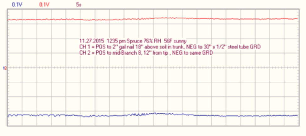

Regarding References 1 and 2, electro-tropism being inhibited by auxin and/or calcium ions, the below 11.27.2015 graph is possible supporting evidence. This voltage recording is of the same spruce tree as shown in Picture 14 and Graphs 15-17. However Channel 2 (red) shows a much more positive voltage (less electrons) at the mid branch than had been observed before. Other recordings at this time were similar everywhere along the branch and other branches as well.

In November of 2015, and at the time of this recording, all the spruce branches were in the natural process of losing needles on the branch interior.

http://forestry.usu.edu/htm/city-and-town/tree-care/my-pine-tree-is-losing-its-needles

This opens the possibility that the tree is purposely restricting the electron flow and that the restricted electron flow is causing the older interior needles to die. Thus the electricity is possibly being manipulated by the auxin or calcium ions. Furthermore, the positive voltage is a possible direct indication of the above mentioned protons, ions, and auxin that are exposed after the electrons are removed.

1. Ishikawa H, Evans ML. Electrotropism of Maize Roots : Role of the Root Cap and Relationship to Gravitropism. PLANT Physiol. 1990;94(3):913-918. doi:10.1104/pp.94.3.913.

2. Nakamura N, Fukushima A, Iwayama H, Suzuki H. Electrotropism of pollen tubes of camellia and other plants. Sex Plant Reprod. 1991;4(2). doi:10.1007/BF00196501.

3. Lucas WJ. Photosynthetic Assimilation of Exogenous HCO3 by Aquatic Plants. Annu Rev Plant Physiol. 1983;34(1):71-104. doi:10.1146/annurev.pp.34.060183. 000443.

4. Walker NA, Smith FA. Circulating Electric Currents Between Acid and Alkaline Zones Associated with HCO – 3 Assimilation in Chara. J Exp Bot. 1977;28(5):1190-1206. doi:10.1093/jxb/28.5.1190.

$C:\Users\Arde\Documents\My PCSGU250\March 2014\10-3-13-232pm-pos-tip-neg-to-ground-rod-spruce-branch5-dead-twig-15-inches-from-trunk.png$

Reviewer No. 2

The paper “Plant Electrotropism” presented by Mr. Ramthun poses an important question of whether the atmospheric electric field of the earth has any contribution to the growth of woody plants. It has an interesting experimental part, where the author has measured the electric properties of plants. Then the author builds a model to evaluate the approximate magnitude of electric forces exerted on a tip of a tree branch. The assumptions that were used are quite simple, and maybe a bit overly simplified, yet the results seem to be reasonable even comparing to a bit more complex approach.

The conclusion that the author makes is that the electric forces might actually govern the growth of a plant, giving it the Lichtenberg-figure type fractal appearance. And this process of electrically governed growth seems to have direct connections to the global electric circuit of earth. The so-called EZ water described in the works of G. Pollack and his co-authors is supposed to have a role in this process.

In my opinion, the results of the described experiments with the horizontal electric field are extremely interesting and deserve to be continued to determine the cause of the plant’s death, as well as the inability of a seed to grow. The apparent tendency of a plant to grow towards the area of space with more positive potential could be an important discovery, verifying the initial hypothesis of the author.

Looking for specific points of possible improvement, I might note the relatively poor introductory part with only a few references.

But in general the paper looks pretty good. It might have important implications not only for biology (concerning the behavior and properties of plants themselves), but also for climatology and weather forecasting (if the plants influence the electric properties of the atmosphere by providing the additional electrons to the atmosphere and thus influencing the condensation nuclei size distribution and cloud formation, and consequently the local energetic balance etc.). This is certainly the work that deserves to be continued.

Here are my comments and questions regarding the specific lines in the text:

Question: In reference to Electric Field Lines of Force lessons learned, I don’t quite understand: how do lines of force affect each other? They are of course parts of a single continuum, but what exactly means for them to affect each other is not clear.

Answer: Repulsed is what I should have said. I replaced “affect” with “repulse” four times.

Question: From my experience (which is quite limited, but still) not every tree grows away from others. Sometimes the adjacent trees “merge” etc. (e.g.: https://goo.gl/IRMF9j). Maybe it is worth considering this case too: what could be the cause of such behavior. (Different electric potentials? Maybe due to different tree species or slightly different mineral/ion content of the soil? Or some interaction with wind and atmospheric electricity – due to geographical orientation: east-west etc.?)

Answer: I also have observed 2 tree trunks in close proximity to each other. A possible explanation is from Dr. Pollack’s book, The Fourth Phase of Water, Chapter 8, A Universal Attractor. The phenomenon is called “like likes like” where like charged particles attract each other. If the tree trunks are close enough to each other, the electrons on each will be pushed away leaving positive charge in the middle which causes the trunks to attract each other.

Question: In the Introduction, maybe the term “Lorentz force” instead of “vector cross product magnetic force” fits here better?

Answer: The Lorentz relation or force is F=q₀E + q₀v x B. The Lorentz force is the combination of electric and magnetic force on A _point charge due to electromagnetic fields. Equation 1 on page 14 is the first half of the Lorentz Force. While I only looked at electric forces, a more thorough analysis should use the entire Lorentz force equation.

Question: Also a comment: were the Lorentz forces the main cause of branching, wouldn’t it happen in one plane only (without axial symmetry of a tree)? I mean, assuming the constant magnetic field direction, the direction of Lorentz force would also be constant given the same electron flow direction. So that would mean that all the branches would lie in one plane and be curved in the same direction. Maybe some kind of such curving (to some degree) indeed is observed? That’s an interesting thing to look into.

Answer: In the Charge Inside the Branch Tip section I added a discussion on branching based on the tip capacitance and charge calculated in Appendix F. In my opinion, as a plant grows, excess charges and electrical forces in the trunk, branch, or leaf cause branching.

Given the electrons and positive ions from EZ water are following the tree branches, they are flowing in many branch directions. Therefore each branch (assuming the branch is straight) and the earth’s magnetic field (B) forms a plane. F is perpendicular to the plane and the magnitude of F = q0vBsinθ. Where v = charge velocity and θ is the included angle between v and B. Charge velocity has not been discussed at all in this paper. Moving charges also create magnetic fields which will interact with the earth’s magnetic field.

Question: In the Introduction about “knocked down” plants. If this process of plant recovery was purely electrostatic, wouldn’t it be pretty fast? Like the motion of electroscope leaves? Maybe the electrostatics here act not as an “acting force,” but more like a “direction sign”giving the general idea of where the plant should move to be healthy again? So it is kind of a “sixth sense,” maybe.

Answer: If there are electrons in the earth and on the plant, then Coulomb force must be present. Small grass is similar in scale to electroscope leaves and grass recovers fast after being knocked over if the damage to the stem is not too severe. For larger plants like corn, the” like likes like” discussed above would happen when the negatively charged plant comes in close proximity to the ground. Also if the plant is touching the ground, the plant will discharge to earth and lose most of its Coulomb repulsive force. As the wound from being folded over heals in the plant stem, negative charge should build just beyond the wound to repulse the plant from the negative earth. An example I have seen of a large tree recovering from getting pushed over is when a palm tree at the shore falls partially over a storm erodes soil away from the roots. The palm responds by bending back to vertical at mid trunk. I expect that is a slow process. I also expect that plants have a level of control of the electrons as possibly demonstrated in the 11-27-2015 recording above.

Question: In the Introduction, you state, “Geotropism and phototropism both fail to explain how neighboring woody plants or plant branches, or blue spruce needles repulse each other.” Is there any specific unexplained effect present?

Answer: I’m talking about plants, plant branches, and needles growing away from each other. The common argument for this effect is “they are growing towards sunlight” But closer observation sees plants and plant parts growing away from sunlight in many cases. Observation also shows every plant and plant part carving out it its own space. Neither geotropism nor phototropism explain how plants to plant, branch to branch, or needle to needle repulsion happens.

Question: I the Introduction, how exactly are branches similar to electric field lines of force? Do they align with them?

Answer: The branches near the top of trees and other woody plants are most clearly similar to the Appendix A, Figure 2 Lines of Force diagram probably because these top branches have clear exposure to the earths electric field positive charges and the trees electric field is directly below the top branches which is also pushing upwards on the branches. As stated in the Abstract and the Resultant Force Discussion, this paper proposes that all of the plant branches are 3D solid copies of electric field lines of force unless gravity or some other physical force changes the plant or branch direction. When a branch loses a smaller branch, the knot left behind causes a physical direction change in the vascular system, water flow and charge flow. The charges follow the water as a conductor, so the electric field line of force also follows the change in branch direction at the knot.

Comment: In the Voltage Recording Discussion, It would also be interesting to know what atmospheric electricity conditions were on the days of measurements. The clouds (and convection in general), for example, might influence the vertical electric current density in the atmosphere and thus alter the readings (supposedly). So the level of humidity, pressure and cloud cover are the things to play with. The atmospheric electricity is also known to depend on the time of day, so that is the other thing to look into. Other thing is geomagnetic conditions, as the geomagnetic storm, for example, might induce currents in the ground and possibly inside the trees themselves. (All of this is more of a suggestion for future work than the remark about this one).

Answer: I agree that much longer voltage recordings using data loggers would probably show relationships not possible with the short term recordings I did.

Comment: In the Voltage Recording Discussion, just a thought: the potential could be less at the tips with the same current density (in order to satisfy the continuity equation) because of the lesser capacitance of the tips (because of their “sharp” pointy shape the charge flows off them more easily, allowing the potential to be smaller).

Answer: Yes I agree. The branches have ends so the current and water is flowing to a “dead end.” The electrons around the bud shown in Figure 26 – Bud Local Charge System will cause both the voltage and electric field to drop around the bud because of increased conductivity. I assume the resistance of air is much greater than the branch and therefore the electrons are slowing down causing the current density to increase at and near the branch tip.

Comment: the current calculated in the Amperage Flowing Towards Branch Tip section is several orders of magnitude bigger than the fair weather vertical electric current density in the atmosphere (picoamperes per square meter).

Answer: That makes sense because the moist branch is a much better conductor than air.

Question: How and why did you arrived at a tip concentration factor?

Answer: The below diagram shows increased charge concentration at a sharp point. This phenomenon is poorly understood.

In Appendix H I calculated the charge concentration based on the buds smaller radius at the tip. I also added the following language from my physics book and charge density calculations:

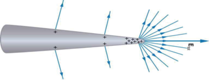
Charge Concentration Illustration²⁷showing positive charge distribution on a sharp point.

“The electric field strength E at points immediately above a charged surface is proportional to the charge density σ so that E may reach very high values near sharp points” ¹³

“If the charged conductor has sharp points, the value of E in the air near the points can be very high.” ¹⁴

Surface charge density (σ). Specifically, σ= q/4πR², where R is the point radius. ¹¹

E also varies by 1/R², specifically

E = F/q₀ = (1/4 πє_o) q / R² ¹²

Question: How are you calculating net tip charge?

Answer: Originally in this paper and my presentations, I had only assumed a charge, but doing your suggested capacitance calculations, I realized the bud could not hold the large charge I had originally assumed. In Appendix H, I assumed the bud is almost neutral except for 2% of extra electrons around the bud and offset by the earth electric field ions pulling and distorting 2% of the electrons towards the incoming earth electric field lines of force. See Figure 26.

Question: It probably should be noted that one thing is some sort of “static” charge at the tip, and the other thing is the current, constantly flowing through it. Which one of those are we dealing with?

Answer: EZ water is sending protonated water to the buds. See Figure 7 and 8. I believe these positive ions are trapped inside the bud leaves or plates. In Appendix F the bud capacitance is calculated using Eq. 6 and actual bud dimensions. These ions are backed up and probably not moving very fast. The electrons on the outside of the branch and tip are attracted to the slow moving ions so they also aren’t moving very fast either. But they are moving or there wouldn’t be an amperage.

Question: What evidence supports this statement? Are any of the known plasma behavior properties observed here? Does it mean that those (supposedly) electrons are in a free state?

Answer: The EZ water process produces separated charges. Protons are being further separated from the electrons by water flow shown in Figures 7 and 8. Whether the charge separation is permanent or temporary is unknown. In order for the electron cloud to reach ne = 1.9 • 10¹⁶ electrons/m³ as calculated in Appendix J, the electrons need to build up for 1.5 hours. However, if the wind blows 1% of the electrons in the electron cloud away, the refresh time is 1 minute. This suggests that some of the electrons are still tied to the protons. Once the electron density within the tree volume reaches a threshold, the new electrons entering will be forced out or be forced farther away from the protons in the bud or leaves. The forced out electrons are then freer to be pulled upwards by the earth’s electric field. I replaced the term “plasma” with “electron cloud.”

Comment: The ionosphere is definitely involved in the same circuit (the global electric circuit). Although I’m not completely sure about VA belts.They are certainly coupled to other current systems (closer to the surface) by electromagnetic induction, but I doubt there is a significant current flowing.

Answer: I don’t know if the Van Allen belts are involved or not, but as I understand, they are large and positively charged.

Question: I think it is worth considering the so-called electrode effect in this context. It basically states that there is a “pillow” of positive charges close to the earth’s surface, since there is a lack of negative charges flowing from downside (there is no downside already; we’re at the surface level) – and positive charges must roughly double to keep the same current density as higher up in the atmosphere. Maybe it could influence the conclusions in some way?

Answer: Yes, In Figure 26, I only showed the local positive charges being attracted to the electrons around the bud and not the longer distance charges.

Comment: I have a suggestion (already made at the conference EU2015: Paths of Discovery in June 2015) that it might be worth repeating those experiments with the light switched off (and then maybe later adding an IR light) to suppress the formation of EZ water and determine whether the potential readings would change.

Answer: Thanks, I have not performed that experiment, but it should be doable.

Comment: In this derivation it seems that only the interaction of 1 m^2 of the ground with the tip is considered, which isn’t quite right. Remember that Coulomb’s law is used for point charges. I would suggest instead to calculate the repulsive force using the Eq. 1 (at 356) taking the E value of an infinite charged plate with the same charge density as the Earth’s. So E = sigma/(2*epsilon_0), where sigma is charge density of aarth (http://farside.ph.utexas.edu/teaching/302l/lectures/node27.html) and thus F = Q_tip*E = Q_tip*sigma/(2*epsilon_0) = 8.1 * 10^(-5) nt. The result is pretty close to the one before, yet pi/2 times bigger.

And please also take note of my comment about Q tip.

Answer: This force calculation is redone in Appendix O. This force (F1) decreased significantly when I decreased the value of Q_tip because I assumed the net charge of both protons and electrons at the tip.

Comment: Here applies the same note about Coulomb’s law as above. It would be better to consider the field of a trunk as a field of a charged cylinder, not A _point charge field. Then the force F = E*Q_tip, and E = 2*k*lambda/r, where k = 9*10^9 nt*m^2/coul^2, r is a distance between the tip and the trunk and lambda is the trunk charge per unit of its length (length = height in this case, so lambda = Q_trunk/H, where H is the height of a trunk, assuming a homogeneous distribution of charge).

Answer: Yes a charged cylinder would be a better model. The point charge was only used for simplifying the model. All of the opposing branch charges were also assumed to be modeled into that single trunk charge.

Another problem here is I don’t think є₀ in k above is proper to use in this model. When I calculated the bud and trunk capacitance in multiple ways, it struck me that nature is optimizing capacitance and charge density. All of the capacitance formulas increased with decreased thickness or diameter of the dielectric between charged surfaces. The narrow water filled xylem tubes seem to fit the parallel conductor capacitance formula. The bud plates seems to fit the plate capacitance formula. Not included in this paper, but the cylindrical capacitance formula applied as multiple coaxial cylinders seems to model the tree rings and the wrapped bud leaves. These capacitance calculations led me to question the accuracy of using є₀ for these force calculation because there is more than free space between the bud and the trunk and nature is not wasteful. I believe all the electrons flowing towards the branch tips and the humidity the plant creates have a purpose in the force calculations. These electrons in Figure 26 create a static electron cloud around the bud and then the incoming electrons form an electron field or plasma that causes a restoring force which directs the bud growth.

While any object that can be electrically charged exhibits capacitance, the theoretical capacitance equations above might need to be modified to model organic plants.

Comment: About the charge of the trunk: it is not obvious that it is 100 times bigger than the charge of the tip. I think the direct observation (or an additional literature review) might be needed to determine the actual measure.

Answer: The factor of 100 was a guess based on the relative size of the trunk/bud. From Appendix F and G, Q_trunk / Qtip plate = -2.0 • 10^-4 coulomb / 2.6 • 10^-7 coulomb = 769.

Comment: To try and evaluate the charge on paper I might recommend only a very rough proxy method: we might assume the same electric potential and different capacitances for the tip and the trunk and determine the charge ratio as Q_tip/Q_trunk = C_tip/C_trunk. To calculate capacitances we might e.g. consider the tip as a small sphere and a trunk as a charged cylinder.

C_tip = R/k = 5.6*10^ (-12) farad (here k = 9*10^9 nt*m^2/coul^2 and I’ve assumed a tip curvature radius R = 0.5 cm).

C_trunk = H/(2*k*ln(r/R)) = 5/(2*9*10^9* ln(1/0.2)) = 1.7*10^(-10) farad (I’ve assumed trunk height H = 5 m, trunk radius R = 0.2 m and also used your assumption of r = 1 m; ln is a natural logarithm function).

(The second equation is derived from the formula for the electric potential of a cylinder:
phi = 2*k*Q_cyl*ln(r/R)/H – it is then substituted to the definition phi = Q_cyl/C_cyl to find C_cyl).

That seems pretty wicked and I’m not sure this is a good way of doing things. But so far I haven’t found any other way. Probably some sort of direct observation might be more reasonable.

Anyway, thus we acquire C_trunk/C_tip = 30, so the charge of the trunk is 30 times bigger. The assumption about 100 times was actually pretty close (maybe even closer to the actual value than this far-fetched calculation). Yet I’ve decided to keep this calculation here anyway.

So to calculate the force we might use again the expression given above, F = 2*k*Q_tip*Q_trunk/ (H*r) = 0.03 nt (I’ve used my number for Q_trunk = 30*Q_tip).

As it can be seen, this value is approximately 10 times smaller than the one acquired in the paper.

Answer: Thank you for helping me understand that capacitance is a good way to estimate charges within the plant. Please see Appendix F where I used plate capacitors to model the bud and Appendix G where I used paired conductors to model the xylem vessels capacitance. Doing capacitance calculations helped me see that plants and plant parts are optimizing capacitance. Thin leaves, thin needles, thin layers, and small diameter vessels all give greater capacitance by how their small thickness and small diameter dimensions minimize the denominator in capacitance equations.

Comment: Again – if the branch has a significant linear size, Coulomb’s law is not the best choice. Although, of course, might serve as a proxy to get the rough order of magnitude. In differential form, however, it might give good results. And again, we have a problem of determining the charge of the branch. This time, however, I won’t make a calculation of my own.

Answer: I came to the conclusion after the Coulomb force calculations in Appendix P and O that Coulomb forces alone would not satisfy this plant growth model. I understood I could not ignore the electrons flowing towards the tips and likely flowing into and accumulating in the air around the plant.

Comment: It would be reasonable to take into account not only the closest 1 cm to the tip, but the whole length of the branch. If the integration seems too wasteful here, it still might be useful to add a fudge factor (something like 1.5 maybe) to put into the equation those parts of the branch sitting further away from the tip. I agree that the charges all along the branch are repulsive to the tip. I made a lot of simplifications to keep the calculations simple.

Answer: I agree, the entire branch could be considered. However, using the Method of Sections procedure allows the forces to be analyzed at any place a section is made. The 1 cm location is where I assumed the branch tip was the most flexible and easy to be bent by directional forces.

If the model is of a branch tip far away from the earth, trunk and other branches, then the forces basically boil down to W, F₄ and F₅. Using the plasma field restoring force F_e, the model also reduces to W, F₄ and F₅ as shown in Appendix M and N.

Question: Isn’t Coulomb’s Force Law (Eq. 1) the same thing as the Electric Field Force (Eq.2)?

Answer: Yes, Thank you. I erroneously assumed the force caused by an electric field and a charge was different and in addition to the action at a distance force between two charges (Coulomb force). Eq. 1 and Eq. 2 are equivalent for stationary charges.

Comment: I don’t think it is reasonable to separate the closest 1 cm and the rest of the branch into different forces.

Answer: I did a force balance on the tip of the branch because it is flexible enough to change direction because lignin hasn’t made the tip rigid yet. I also used 1 cm to keep the Coulomb force from being too large based on my charge assumptions. A smaller charge at the tip is possible and could result in the same Coulomb force if the 1 cm distance is decreased.

Comment: If we assume the area of branch cross-section of 1 cm^2, this force would create tension of about 3*10^4 Pa, which is two orders of magnitude lower than the pressure inside the big trees trunks (maybe a literature review might show otherwise? I’m not sure). This is a possible argument against the idea that the growth itself is caused by the electrical forces. It might, however, be subtly directed by them.

Answer: I think a branch or twig cross sectional area near A _bud is somewhat smaller than 1 cm². Looking at actual twigs, I estimate the twig diameter to be 3/16” or .48 cm. This calculates to be a cross sectional area of 0.178 cm². So the two orders of magnitude factor is reduced to 20. The pressure inside of the trunk needs to be greater than at the tip to get water to flow towards the tip. In other words, there is a pressure drop between the trunk and the tip. Also as I mentioned above, the distance of 1 cm between the tip charge and the branch charge was needed to keep the repulsive Coulomb force reasonable. Even if the tip charge is reduced by a factor of 10, the force within the tip could be 100 times larger if the distance between charges is reduced from 1 cm to 0.1 mm.

Because the trunk loses protons to the buds continuously from EZ Water, the electrons inside the trunk outnumber the ions. This creates an electron restoring force F_e inside the trunk and branches which is probably the cause of tree ring growth.

The below link suggests electric fields give direction to plant growth as you suggested.

http://www.ncbi.nlm.nih.gov/pubmed/ 12879446

Reviewer No.2 – Second Review

Question: Is FM satellite radio interference and GPS satellite signal interference near or under trees a known fact or an observation made by the author? Maybe a reference link is needed?

Potentially this seems to be an important discovery. This effect should be studied further.

Answer: Both of these radio wave interferences have been my observation. After purchasing a new car with satellite radio, my wife and I went on a fall color tour drive. We both noticed the radio cutting out beneath large trees.

At my job, we do many survey grade GPS surveys. The base station receives GPS satellites signals and is always set up in an open area. However, the rover or data collector also receives GPS satellite signals, and often loses signal when taking survey shots near large trees.

See Appendix K – Electron Cloud Frequency.

I added a link mentioning the tree interference problem ⁴³ See two posts mid-page.

Question: Are the concentrations of these charged particles (with respect to the neutral air molecules) enough to call it a plasma?

Answer: In Appendix J, my estimate of the electron density within the tree volume is 1.9 x 1016 electrons/m³ (1.9 x10¹⁰ electrons/cm³). From the plasma link³⁹ , the ionosphere is 10¹⁰ particles/cm³ and the atmosphere at sea level is 10¹⁹ molecules/cm³. So 10¹⁹/10¹⁰ = approximately 1 billion air molecules/electron. I changed plasma to electron cloud.

If the electron cloud is not a plasma, I believe it could be behaving like a plasma in spite of all the neutral air molecules. Possibly, this is where polarized humidity droplets are an important force transmitting part of the electron cloud.

Question: Very interesting point. Indeed the presence of water might significantly change the picture. Maybe it is possible to make some comparison to the plants growing in more arid areas (deserts, etc.) to see if we should observe different morphology due to the lower water abundance?

Answer: Doing the capacitance calculations, it struck me that plants are optimizing their environment to achieve growth, which would include the humidity field they create around themselves when they transpire water. Optimizing their electrical environment would therefore go beyond Coulomb forces and should include the probable charges in the air near the tree. Not considered at all here are magnetic forces which in my opinion could be what sometimes gives some trees a “twisted trunk.”

I had not thought about comparing plants in different humidity conditions to see if there is an observable difference in plant growth based on humidity.

Thank you very much to both reviewers for your help and insightful questions!